Note: This is an auto-generated Markdown version of the Jupyter notebook MercuryRemoval_LNG_Pretreatment.ipynb. You can also view it on nbviewer or open it in Google Colab.

---

Purpose and engineering boundary

This notebook demonstrates the public MercuryRemovalBed API with a synthetic gas case. It separates configured inputs from calculated results and checks internal model behaviour. It is an educational screening workflow, not a vendor guarantee, a plant-performance prediction, or an approved pressure-vessel or cost estimate.

The model represents irreversible fixed-bed chemisorption of elemental mercury. A simplified reaction concept is:

\[\mathrm{Hg^0 + CuS \rightarrow HgS + Cu}\]

Actual sorbent selection, capacity, kinetics, replacement utilisation, vessel design, and cost basis require supplier data and accountable engineering review for the project conditions.

Workflow

1. create a synthetic trace-mercury feed and document the normal-volume basis;
2. calculate steady removal, pressure drop, inventory, and capacity-based lifetime;
3. run an accelerated transient example and inspect loading profiles;
4. explore configured degradation and pre-loading scenarios;
5. inspect serializable JSON outputs;
6. run preliminary mechanical and cost screening;
7. verify boundedness, monotonic trends, and configuration diagnostics.

Setup and imports

The setup cell installs the released public-PyPI package only when neqsim is absent, so it works in a clean Google Colab runtime while remaining quiet in an already prepared environment. The saved execution below used NeqSim 3.17.0; reruns report the actual Python, Java, and package versions.

import importlib.util

if importlib.util.find_spec("neqsim") is None:
    %pip install -q "neqsim==3.17.0"

import importlib.metadata
import json
import platform

import matplotlib.pyplot as plt
import numpy as np
from neqsim import jneqsim
from jpype import JClass

SystemSrkEos = jneqsim.thermo.system.SystemSrkEos
Stream = jneqsim.process.equipment.stream.Stream
MercuryRemovalBed = jneqsim.process.equipment.adsorber.MercuryRemovalBed
UUID = JClass("java.util.UUID")
JavaSystem = JClass("java.lang.System")

neqsim_version = importlib.metadata.version("neqsim")
java_version = str(JavaSystem.getProperty("java.version"))

print(f"Python: {platform.python_version()}")
print(f"Java: {java_version}")
print(f"NeqSim: {neqsim_version}")

Output

``` Python: 3.12.13 Java: 17.0.19 NeqSim: 3.17.0 ```

Part 1: Create a synthetic feed with trace mercury

The component amounts below define a reproducible teaching case, not a named field or LNG train. NeqSim normalizes them to mole fractions. Mercury concentration is reported on a stated normal basis of 0 °C and 1.01325 bar, using 44.615 mol/Nm³ and a mercury molar mass of 200.59 g/mol:

\[c_{\mathrm{Hg},N}=x_{\mathrm{Hg}}\rho_{N,\mathrm{mol}}M_{\mathrm{Hg}}10^6\]

Here $c_{\mathrm{Hg},N}$ is in µg/Nm³, $x_{\mathrm{Hg}}$ is mole fraction, $\rho_{N,\mathrm{mol}}$ is mol/Nm³, and $M_{\mathrm{Hg}}$ is g/mol. This explicit conversion avoids mixing process-volume and normal-volume concentration bases.

# Synthetic gas at 30 °C and 60 bara
feed_gas = SystemSrkEos(303.15, 60.0)
feed_gas.addComponent("methane", 0.85)
feed_gas.addComponent("ethane", 0.07)
feed_gas.addComponent("propane", 0.03)
feed_gas.addComponent("nitrogen", 0.04)
feed_gas.addComponent("CO2", 0.005)
feed_gas.addComponent("mercury", 2.0e-8)
feed_gas.createDatabase(True)
feed_gas.setMixingRule(2)
feed_gas.init(0)

feed = Stream("LNG Feed", feed_gas)
feed.setFlowRate(100000.0, "kg/hr")
feed.run()

normal_molar_density = 44.615
mercury_molar_mass = 200.59
x_hg = float(feed_gas.getPhase(0).getComponent("mercury").getx())
c_hg_ntp = x_hg * normal_molar_density * mercury_molar_mass * 1.0e6

print("=== Synthetic feed conditions ===")
print(f"Temperature: {feed.getTemperature() - 273.15:.1f} °C")
print(f"Pressure: {feed.getPressure():.1f} bara")
print(f"Mass flow: {feed.getFlowRate('kg/hr'):.0f} kg/h")
print(f"Gas density: {feed.getThermoSystem().getPhase(0).getDensity('kg/m3'):.2f} kg/m³")
print(f"Mercury mole fraction: {x_hg:.6e}")
print(f"Mercury concentration at 0 °C, 1.01325 bar: {c_hg_ntp:.2f} µg/Nm³")

Output

``` === Synthetic feed conditions === Temperature: 30.0 °C Pressure: 60.0 bara Mass flow: 100000 kg/h Gas density: 49.63 kg/m³ Mercury mole fraction: 2.010050e-08 Mercury concentration at 0 °C, 1.01325 bar: 179.89 µg/Nm³ ```

Part 2: Configure and run steady-state mercury removal

Geometry, sorbent properties, kinetics, degradation, and replacement utilisation are user inputs. They are not inferred or validated against a vendor product by this example. The steady calculation uses the current NeqSim NTU/kinetic model and Ergun pressure-drop implementation.

hg_bed = MercuryRemovalBed("Mercury Guard Bed", feed)

# Configured geometry
hg_bed.setBedDiameter(2.0)
hg_bed.setBedLength(5.0)
hg_bed.setVoidFraction(0.40)
hg_bed.setParticleDiameter(0.004)

# Configured sorbent and kinetic screening inputs
hg_bed.setSorbentType("PuraSpec")
hg_bed.setSorbentBulkDensity(1100.0)
hg_bed.setMaxMercuryCapacity(100000.0)
hg_bed.setReactionRateConstant(0.5)
hg_bed.setActivationEnergy(25000.0)
hg_bed.setReferenceTemperature(298.15)
hg_bed.setDegradationFactor(1.0)
hg_bed.setBypassFraction(0.0)
hg_bed.setReplacementUtilisation(0.50)

hg_bed.run(UUID.randomUUID())

removal_efficiency = float(hg_bed.getRemovalEfficiency())
pressure_drop_bar = float(hg_bed.getPressureDrop("bar"))
estimated_lifetime_hours = float(hg_bed.estimateBedLifetime())
estimated_lifetime_years = estimated_lifetime_hours / 8760.0

print("=== Steady-state screening results ===")
print(f"Removal efficiency: {removal_efficiency * 100:.2f} %")
print(f"Pressure drop: {pressure_drop_bar:.4f} bar")
print(f"Sorbent mass: {hg_bed.getSorbentMass():.0f} kg")
print(f"Bed volume: {hg_bed.getBedVolume():.2f} m³")
print(f"Capacity-based lifetime: {estimated_lifetime_hours:.0f} h")
print(f"Capacity-based lifetime: {estimated_lifetime_years:.2f} years")
print(f"Replacement utilisation input: {hg_bed.getReplacementUtilisation():.2f}")

outlet = hg_bed.getOutletStream()
print(f"Outlet temperature: {outlet.getTemperature() - 273.15:.1f} °C")
print(f"Outlet pressure: {outlet.getPressure():.2f} bara")

Output

``` === Steady-state screening results === Removal efficiency: 99.87 % Pressure drop: 0.3292 bar Sorbent mass: 10367 kg Bed volume: 15.71 m³ Capacity-based lifetime: 23781 h Capacity-based lifetime: 2.71 years Replacement utilisation input: 0.50 Outlet temperature: 30.0 °C Outlet pressure: 59.67 bara ```

Part 3: Accelerated transient loading example

Transient mode tracks local sorbent loading and gas-phase mercury concentration in axial cells. The internal rate form is represented conceptually by:

\[r=k_{\mathrm{eff}}C_{\mathrm{Hg}}(1-\theta)\]

where $\theta=q/q_{\max}$ is fractional loading. To make the state evolution visible in a short notebook run, this section deliberately uses a higher mercury amount than Part 1. Its time scale is therefore a numerical demonstration and must not be interpreted as service life for a real bed.

# Deliberately elevated mercury amount for an accelerated numerical demonstration
high_hg_gas = SystemSrkEos(273.15 + 30.0, 60.0)
high_hg_gas.addComponent("methane", 0.85)
high_hg_gas.addComponent("ethane", 0.07)
high_hg_gas.addComponent("propane", 0.03)
high_hg_gas.addComponent("nitrogen", 0.04)
high_hg_gas.addComponent("CO2", 0.005)
high_hg_gas.addComponent("mercury", 1.0e-6)
high_hg_gas.createDatabase(True)
high_hg_gas.setMixingRule(2)
high_hg_gas.init(0)

high_hg_feed = Stream("High Hg Feed", high_hg_gas)
high_hg_feed.setFlowRate(100000.0, "kg/hr")
high_hg_feed.run()

# Configure for transient simulation
hg_bed_transient = MercuryRemovalBed("Hg Bed Transient", high_hg_feed)
hg_bed_transient.setBedDiameter(2.0)
hg_bed_transient.setBedLength(5.0)
hg_bed_transient.setVoidFraction(0.40)
hg_bed_transient.setParticleDiameter(0.004)
hg_bed_transient.setSorbentType("PuraSpec")
hg_bed_transient.setSorbentBulkDensity(1100.0)
hg_bed_transient.setMaxMercuryCapacity(100000.0)
hg_bed_transient.setReactionRateConstant(0.5)
hg_bed_transient.setNumberOfCells(30)
hg_bed_transient.setCalculatePressureDrop(False)
hg_bed_transient.setBreakthroughThreshold(0.01)

# IMPORTANT: Disable steady-state to enable cell-by-cell transient
hg_bed_transient.setCalculateSteadyState(False)
hg_bed_transient.initialiseTransientGrid()

# Time-stepping: simulate 2000 hours in 100-hour steps
calc_id = UUID.randomUUID()
dt_seconds = 100.0 * 3600  # 100 hours per step
n_steps = 20

# Track results
times = []
avg_loadings = []
utilisations = []
breakthrough_status = []

print("Time (h)  | Avg Loading (mg/kg) | Utilisation (%) | Breakthrough")
print("-" * 70)

for step in range(n_steps):
    hg_bed_transient.runTransient(dt_seconds, calc_id)

    t = hg_bed_transient.getElapsedTimeHours()
    q_avg = hg_bed_transient.getAverageLoading()
    util = hg_bed_transient.getBedUtilisation()
    bt = hg_bed_transient.isBreakthroughOccurred()

    times.append(t)
    avg_loadings.append(q_avg)
    utilisations.append(util * 100)
    breakthrough_status.append(bt)

    print(f"{t:9.0f} | {q_avg:19.1f} | {util * 100:15.2f} | {'YES' if bt else 'No'}")

bt_hrs = hg_bed_transient.getBreakthroughTimeHours()
print(f"\nBreakthrough time: {bt_hrs:.0f} hours" if bt_hrs > 0 else "\nNo breakthrough during simulation")

Output

``` Time (h) | Avg Loading (mg/kg) | Utilisation (%) | Breakthrough ---------------------------------------------------------------------- 100 | 10499.6 | 10.50 | No 200 | 20984.2 | 20.98 | No 300 | 31437.2 | 31.44 | No 400 | 41823.8 | 41.82 | YES 500 | 52073.0 | 52.07 | YES 600 | 62044.4 | 62.04 | YES 700 | 71479.8 | 71.48 | YES 800 | 79967.1 | 79.97 | YES 900 | 87001.7 | 87.00 | YES 1000 | 92220.9 | 92.22 | YES 1100 | 95653.8 | 95.65 | YES 1200 | 97687.9 | 97.69 | YES 1300 | 98806.7 | 98.81 | YES 1400 | 99394.5 | 99.39 | YES 1500 | 99695.5 | 99.70 | YES 1600 | 99847.6 | 99.85 | YES 1700 | 99923.9 | 99.92 | YES 1800 | 99962.0 | 99.96 | YES 1900 | 99981.1 | 99.98 | YES 2000 | 99990.6 | 99.99 | YES Breakthrough time: 300 hours ```

# Plot bed loading and utilisation over time
fig, (ax1, ax2) = plt.subplots(1, 2, figsize=(14, 5))

# Average loading vs time
ax1.plot(times, avg_loadings, 'b-o', linewidth=2, markersize=4)
ax1.set_xlabel('Time on Stream (hours)', fontsize=12)
ax1.set_ylabel('Average Loading (mg Hg / kg sorbent)', fontsize=12)
ax1.set_title('Bed Loading Over Time', fontsize=14)
ax1.grid(True, alpha=0.3)
ax1.axhline(y=hg_bed_transient.getMaxMercuryCapacity(), color='r', linestyle='--',
            label=f'Max capacity ({hg_bed_transient.getMaxMercuryCapacity():.0f} mg/kg)')
ax1.legend()

# Utilisation vs time
ax2.plot(times, utilisations, 'g-o', linewidth=2, markersize=4)
ax2.set_xlabel('Time on Stream (hours)', fontsize=12)
ax2.set_ylabel('Bed Utilisation (%)', fontsize=12)
ax2.set_title('Bed Utilisation Over Time', fontsize=14)
ax2.grid(True, alpha=0.3)

# Mark breakthrough if it occurred
bt_time = hg_bed_transient.getBreakthroughTimeHours()
if bt_time > 0:
    ax2.axvline(x=bt_time, color='r', linestyle='--', label=f'Breakthrough at {bt_time:.0f} h')
    ax2.legend()

plt.tight_layout()
plt.savefig('mercury_bed_loading.png', dpi=150, bbox_inches='tight')
plt.show()
print("Plot saved to mercury_bed_loading.png")

Output

``` Plot saved to mercury_bed_loading.png ```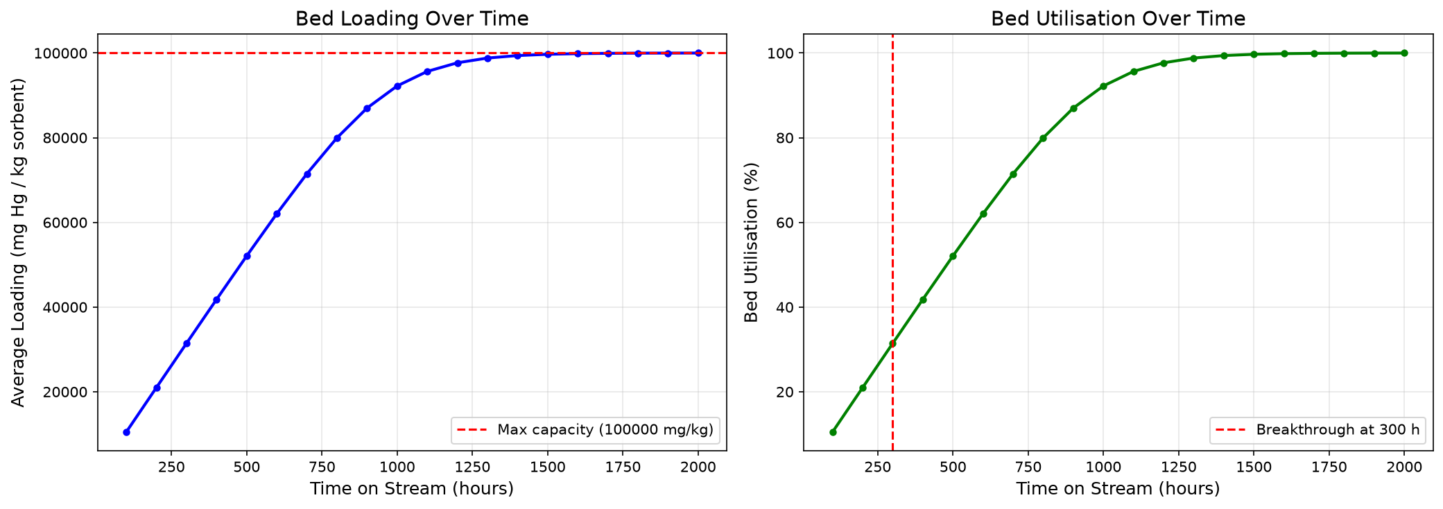

Part 4: Axial loading profile

The profiles expose the state of each discretized axial cell. They are model outputs for the accelerated case. A real mass-transfer-zone length requires calibrated kinetics, dispersion, sorbent data, and representative inlet conditions.

# Get the loading and concentration profiles
loading_profile = list(hg_bed_transient.getLoadingProfile())
conc_profile = list(hg_bed_transient.getConcentrationProfile())
n_cells = hg_bed_transient.getNumberOfCells()
positions = np.linspace(0, hg_bed_transient.getBedLength(), n_cells)

fig, (ax1, ax2) = plt.subplots(2, 1, figsize=(12, 8))

# Loading profile
ax1.bar(positions, loading_profile, width=positions[1] - positions[0],
        color='steelblue', alpha=0.7, edgecolor='navy')
ax1.set_xlabel('Axial Position (m)', fontsize=12)
ax1.set_ylabel('Loading (mg Hg / kg sorbent)', fontsize=12)
ax1.set_title(f'Mercury Loading Profile at {hg_bed_transient.getElapsedTimeHours():.0f} hours', fontsize=14)
ax1.axhline(y=hg_bed_transient.getMaxMercuryCapacity(), color='r', linestyle='--',
            label='Maximum capacity')
ax1.legend()
ax1.grid(True, alpha=0.3)

# Concentration profile
ax2.plot(positions, conc_profile, 'r-o', linewidth=2, markersize=4)
ax2.set_xlabel('Axial Position (m)', fontsize=12)
ax2.set_ylabel('Gas-Phase Hg Conc. (µg/Nm³)', fontsize=12)
ax2.set_title('Gas-Phase Mercury Concentration Along the Bed', fontsize=14)
ax2.grid(True, alpha=0.3)

plt.tight_layout()
plt.savefig('mercury_axial_profiles.png', dpi=150, bbox_inches='tight')
plt.show()

# Mass transfer zone length
mtz = hg_bed_transient.getMassTransferZoneLength()
print(f"Mass Transfer Zone (MTZ) length: {mtz:.2f} m")
print(f"Bed length: {hg_bed_transient.getBedLength():.1f} m")
if mtz > 0:
    print(f"MTZ as fraction of bed: {mtz / hg_bed_transient.getBedLength() * 100:.1f}%")

Output

``` Mass Transfer Zone (MTZ) length: 0.00 m Bed length: 5.0 m ```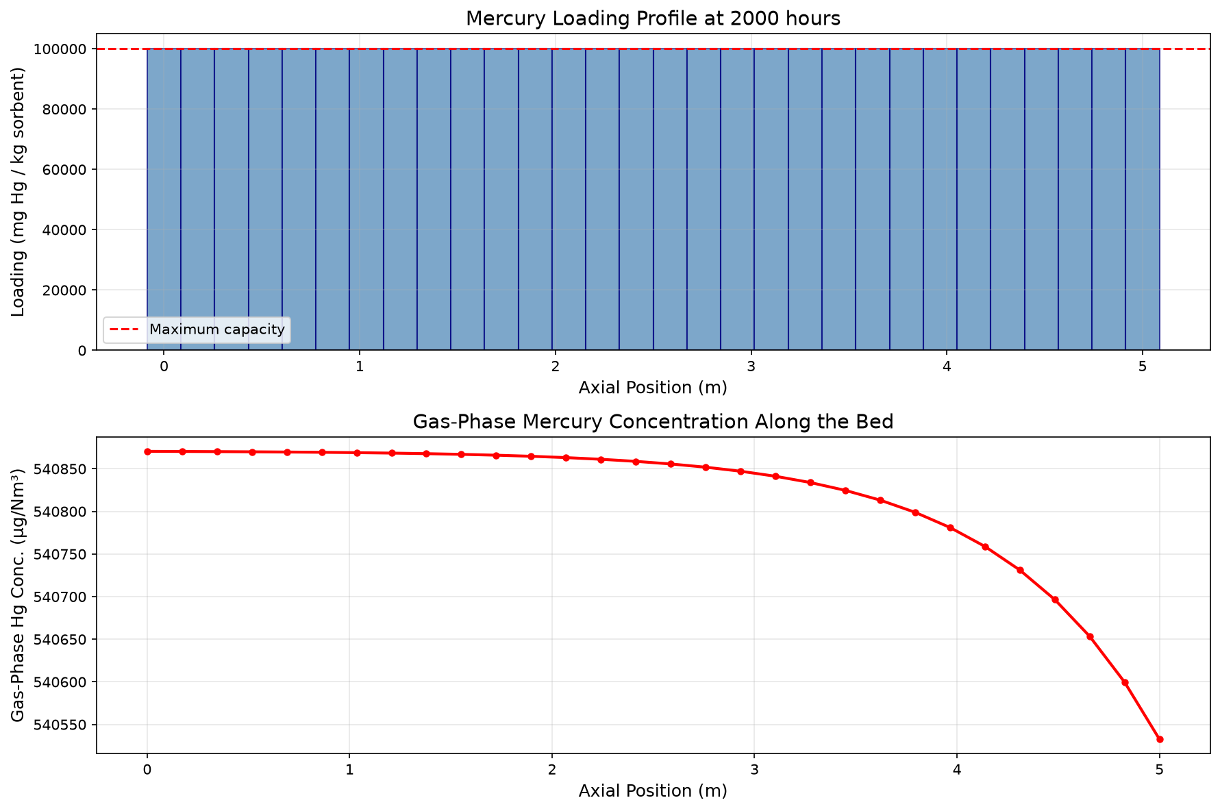

Part 5: Configured degradation sensitivity

degradationFactor and bypassFraction are scenario controls, not condition-monitoring estimates. The comparison below verifies the direction of the configured model response. It does not predict damage probability, diagnose internals, or replace inspection data.

Input	Model role
degradationFactor	scales effective capacity and kinetic rate
bypassFraction	sends a configured fraction around the sorbent response

# Compare fresh vs degraded bed performance
scenarios = [
    {"name": "Fresh bed",              "degradation": 1.0, "bypass": 0.0},
    {"name": "Mild fouling",           "degradation": 0.8, "bypass": 0.05},
    {"name": "Moderate degradation",   "degradation": 0.6, "bypass": 0.10},
    {"name": "Severe channelling",     "degradation": 0.4, "bypass": 0.20},
]

print(f"{'Scenario':<25} | {'Efficiency (%)':<15} | {'ΔP (mbar)':<12} | {'Lifetime (yr)':<14}")
print("-" * 72)

efficiencies = []
labels = []

for sc in scenarios:
    bed = MercuryRemovalBed("Hg_" + sc["name"], feed)
    bed.setBedDiameter(2.0)
    bed.setBedLength(5.0)
    bed.setVoidFraction(0.40)
    bed.setParticleDiameter(0.004)
    bed.setSorbentType("PuraSpec")
    bed.setSorbentBulkDensity(1100.0)
    bed.setMaxMercuryCapacity(100000.0)
    bed.setReactionRateConstant(0.5)
    bed.setDegradationFactor(float(sc["degradation"]))
    bed.setBypassFraction(float(sc["bypass"]))
    bed.setReplacementUtilisation(0.50)
    bed.run(UUID.randomUUID())

    eff = bed.getRemovalEfficiency() * 100
    dp = bed.getPressureDrop() / 100  # Pa to mbar
    lifetime = bed.estimateBedLifetime() / 8760  # hours to years

    efficiencies.append(eff)
    labels.append(sc["name"])

    print(f"{sc['name']:<25} | {eff:<15.2f} | {dp:<12.1f} | {lifetime:<14.1f}")

# Bar chart
fig, ax = plt.subplots(figsize=(10, 5))
colors = ['#2ecc71', '#f1c40f', '#e67e22', '#e74c3c']
bars = ax.bar(labels, efficiencies, color=colors, edgecolor='black', alpha=0.8)
ax.set_ylabel('Mercury Removal Efficiency (%)', fontsize=12)
ax.set_title('Impact of Column Degradation on Mercury Removal', fontsize=14)
ax.set_ylim(0, 105)
ax.grid(True, alpha=0.3, axis='y')

for bar, eff in zip(bars, efficiencies):
    ax.text(bar.get_x() + bar.get_width() / 2, bar.get_height() + 1,
            f'{eff:.1f}%', ha='center', fontsize=11, fontweight='bold')

plt.tight_layout()
plt.savefig('mercury_degradation_impact.png', dpi=150, bbox_inches='tight')
plt.show()

Output

``` Scenario | Efficiency (%) | ΔP (mbar) | Lifetime (yr) ------------------------------------------------------------------------ Fresh bed | 99.87 | 329.2 | 2.7 Mild fouling | 94.53 | 329.2 | 2.2 Moderate degradation | 88.31 | 329.2 | 1.6 Severe channelling | 74.36 | 329.2 | 1.1 ```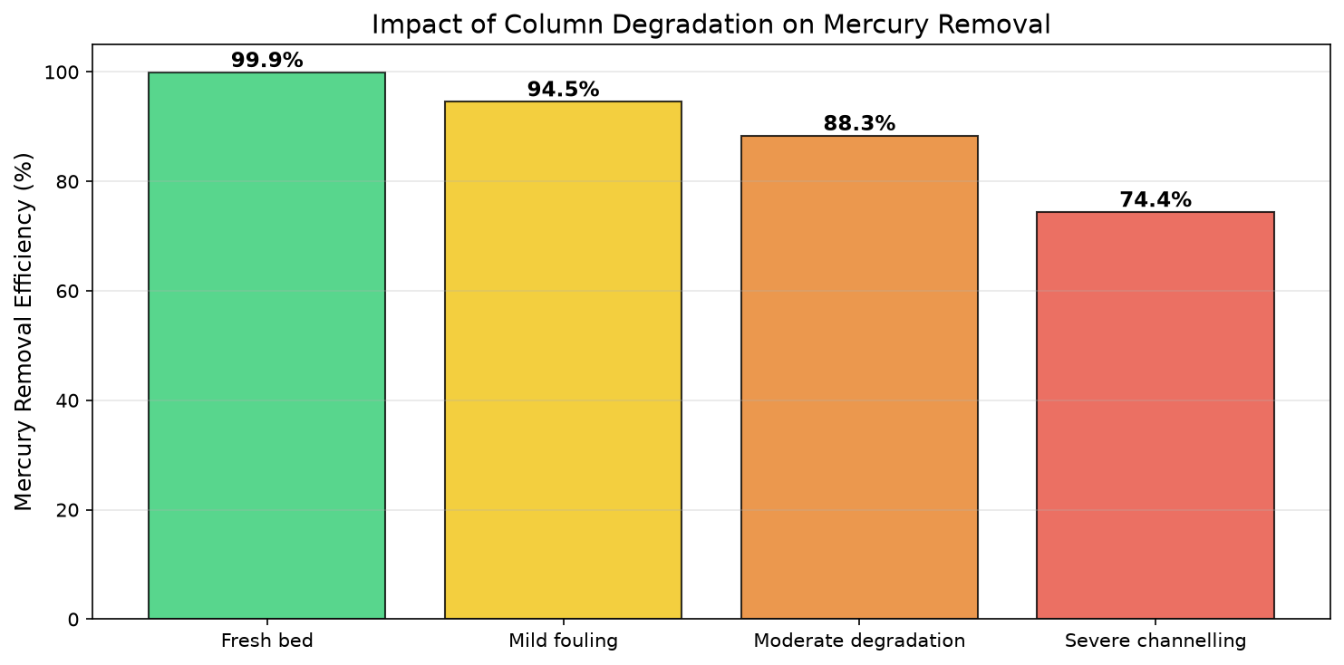

Part 6: Bed pre-loading

preloadBed() initializes a uniform spent fraction for restart and sensitivity studies. It does not reconstruct a measured loading profile. The accelerated feed is retained so the remaining capacity evolves within the notebook runtime.

# Simulate a bed already 80% spent, using the elevated-Hg feed
hg_preloaded = MercuryRemovalBed("Preloaded Bed", high_hg_feed)
hg_preloaded.setBedDiameter(2.0)
hg_preloaded.setBedLength(5.0)
hg_preloaded.setVoidFraction(0.40)
hg_preloaded.setParticleDiameter(0.004)
hg_preloaded.setSorbentType("PuraSpec")
hg_preloaded.setSorbentBulkDensity(1100.0)
hg_preloaded.setMaxMercuryCapacity(100000.0)
hg_preloaded.setReactionRateConstant(0.5)
hg_preloaded.setNumberOfCells(30)
hg_preloaded.setCalculatePressureDrop(False)
hg_preloaded.setCalculateSteadyState(False)

# Pre-load to 80% of capacity
hg_preloaded.preloadBed(0.80)
print(f"Initial average loading: {hg_preloaded.getAverageLoading():.0f} mg/kg")
print(f"Initial utilisation:     {hg_preloaded.getBedUtilisation() * 100:.1f}%")

# Run for 1000 hours and see how quickly it saturates
calc_id = UUID.randomUUID()
preload_times = []
preload_utils = []

for step in range(20):
    hg_preloaded.runTransient(50.0 * 3600, calc_id)
    preload_times.append(hg_preloaded.getElapsedTimeHours())
    preload_utils.append(hg_preloaded.getBedUtilisation() * 100)

print(f"\nFinal utilisation after {hg_preloaded.getElapsedTimeHours():.0f} hours: "
      f"{hg_preloaded.getBedUtilisation() * 100:.1f}%")
print(f"Breakthrough occurred: {hg_preloaded.isBreakthroughOccurred()}")
if hg_preloaded.getBreakthroughTimeHours() > 0:
    print(f"Breakthrough time: {hg_preloaded.getBreakthroughTimeHours():.0f} hours")

# Plot
fig, ax = plt.subplots(figsize=(10, 5))
ax.plot(preload_times, preload_utils, 'r-o', linewidth=2, markersize=4)
ax.set_xlabel('Time on Stream (hours)', fontsize=12)
ax.set_ylabel('Bed Utilisation (%)', fontsize=12)
ax.set_title('Remaining Capacity of an 80% Pre-Loaded Bed', fontsize=14)
ax.axhline(y=100, color='k', linestyle='--', alpha=0.5, label='Fully spent')
ax.grid(True, alpha=0.3)
ax.legend()
plt.tight_layout()
plt.show()

Output

``` Initial average loading: 80000 mg/kg Initial utilisation: 80.0% Final utilisation after 1000 hours: 100.0% Breakthrough occurred: True ```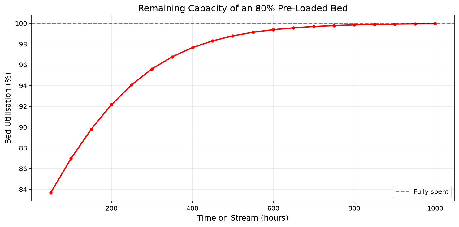

Part 7: JSON reporting

The equipment JSON retains stable names, explicit field units, configured inputs, and calculated state for logging or downstream serialization. It does not add measurement provenance or approve the values for a digital-twin acceptance workflow.

# Get JSON report from the steady-state bed
hg_bed.run(UUID.randomUUID())
report = json.loads(str(hg_bed.toJson()))

print("=== Mercury Removal Bed — JSON Report ===")
print(json.dumps(report, indent=2))

Output

``` === Mercury Removal Bed — JSON Report === { "name": "Mercury Guard Bed", "equipmentType": "MercuryRemovalBed", "geometry": { "bedDiameter_m": 2.0, "bedLength_m": 5.0, "bedVolume_m3": 15.707963267948966, "voidFraction": 0.4, "particleDiameter_m": 0.004 }, "sorbent": { "type": "PuraSpec", "bulkDensity_kg_m3": 1100.0, "totalMass_kg": 10367.255756846318, "maxMercuryCapacity_mg_per_kg": 100000.0 }, "kinetics": { "reactionRateConstant_1_per_s": 0.5, "activationEnergy_J_per_mol": 25000.0, "referenceTemperature_K": 298.15 }, "degradation": { "degradationFactor": 1.0, "bypassFraction": 0.0, "replacementUtilisation": 0.5 }, "operating": { "elapsedTime_hours": 0.0, "pressureDrop_Pa": 32916.077346093254, "averageLoading_mg_per_kg": 0.0, "bedUtilisation": 0.0, "breakthroughOccurred": false, "estimatedLifetime_hours": 23780.95436405089 } } ```

Part 8: Preliminary mechanical screening

MercuryRemovalMechanicalDesign applies a simplified hoop-stress fallback and empirical weight factors. The reported standard-code string and material label are metadata; this calculation does not demonstrate ASME Section VIII compliance. It omits, among other requirements, a governed material-temperature basis, corrosion allowance, external pressure, nozzle and local loads, fatigue, supports, fabrication details, inspection, testing, and accountable code review.

Use these outputs only for early screening. A project vessel must be designed and verified under the applicable code and jurisdiction by qualified engineers.

# Create mechanical design from the steady-state bed
mech_design = hg_bed.getMechanicalDesign()
mech_design.setMaxOperationPressure(60.0)       # 60 bara design pressure
mech_design.setMaxOperationTemperature(273.15 + 80.0)  # 80°C

# Run the design calculation
mech_design.calcDesign()

# Print results
print("=== Preliminary mechanical-screening results ===")
print(f"Inner diameter:      {mech_design.innerDiameter:.2f} m")
print(f"Outer diameter:      {mech_design.getOuterDiameter():.4f} m")
print(f"Wall thickness:      {mech_design.getWallThickness():.1f} mm")
print(f"Tan-tan length:      {mech_design.tantanLength:.2f} m")
print(f"Material grade:      {mech_design.getMaterialGrade()}")
print(f"\n--- Weight Breakdown ---")
print(f"Vessel shell:        {mech_design.getWeigthVesselShell():.0f} kg")
print(f"Internals:           {mech_design.getInternalsWeight():.0f} kg")
print(f"Sorbent charge:      {mech_design.getSorbentChargeWeight():.0f} kg")
print(f"Nozzles:             {mech_design.getWeightNozzle():.0f} kg")
print(f"Piping:              {mech_design.getWeightPiping():.0f} kg")
print(f"Structural steel:    {mech_design.getWeightStructualSteel():.0f} kg")
print(f"Electrical/instr:    {mech_design.getWeightElectroInstrument():.0f} kg")
print(f"TOTAL skid weight:   {mech_design.getWeightTotal():.0f} kg")
print(f"\n--- Module Footprint ---")
print(f"Width:  {mech_design.getModuleWidth():.1f} m")
print(f"Length: {mech_design.getModuleLength():.1f} m")
print(f"Height: {mech_design.getModuleHeight():.1f} m")

Output

``` === Preliminary mechanical-screening results === Inner diameter: 2.00 m Outer diameter: 2.1159 m Wall thickness: 57.9 mm Tan-tan length: 7.00 m Material grade: SA-516-70 --- Weight Breakdown --- Vessel shell: 25956 kg Internals: 668 kg Sorbent charge: 10367 kg Nozzles: 1298 kg Piping: 10382 kg Structural steel: 2596 kg Electrical/instr: 2076 kg TOTAL skid weight: 42977 kg --- Module Footprint --- Width: 4.0 m Length: 5.0 m Height: 8.0 m ```

# Bill of Materials
bom = mech_design.generateBillOfMaterials()
print("=== Bill of Materials ===")
print(f"{'Item':<40} | {'Material':<15} | {'Weight (kg)':<12}")
print("-" * 72)
for item in bom:
    name = str(item.get("item"))
    material = str(item.get("material"))
    weight = float(str(item.get("weight_kg")))
    print(f"{name:<40} | {material:<15} | {weight:<12.0f}")

Output

``` === Bill of Materials === Item | Material | Weight (kg) ------------------------------------------------------------------------ Pressure Vessel Shell | SA-516-70 | 25956 Sorbent Charge (PuraSpec) | PuraSpec | 10367 Support Grids and Distribution Plates | SS316L | 668 Inlet/Outlet Nozzles | SA-516-70 | 1298 ```

# Full mechanical design JSON report
mech_json = json.loads(str(mech_design.toJson()))
print("=== Mechanical Design — Full JSON Report ===")
print(json.dumps(mech_json, indent=2))

Output

``` === Mechanical Design — Full JSON Report === { "equipmentName": "Mercury Guard Bed", "equipmentType": "MercuryRemovalBed", "designStandardCode": "ASME-VIII-Div1", "materialGrade": "SA-516-70", "geometry": { "innerDiameter_m": 2.0, "outerDiameter_m": 2.115875872360971, "wallThickness_mm": 57.93793618048545, "tanTanLength_m": 7.0 }, "weights": { "emptyVesselShell_kg": 25956.195408857486, "internals_kg": 668.3627878423159, "sorbentCharge_kg": 10367.255756846318, "nozzles_kg": 1297.8097704428744, "piping_kg": 10382.478163542995, "structural_kg": 2595.619540885749, "electrical_kg": 2076.495632708599, "totalSkid_kg": 42976.96130428001 }, "footprint": { "width_m": 4.0, "length_m": 5.0, "height_m": 8.0 }, "billOfMaterials": [ { "item": "Pressure Vessel Shell", "material": "SA-516-70", "weight_kg": 25956.195408857486 }, { "item": "Sorbent Charge (PuraSpec)", "material": "PuraSpec", "weight_kg": 10367.255756846318 }, { "item": "Support Grids and Distribution Plates", "material": "SS316L", "weight_kg": 668.3627878423159 }, { "item": "Inlet/Outlet Nozzles", "material": "SA-516-70", "weight_kg": 1297.8097704428744 } ] } ```

Part 9: Preliminary cost-factor screening

The cost class combines weight-based steel, sorbent price, module factors, and maintenance factors. The numerical results are unindexed nominal USD from editable class defaults. No cost year, location, currency date, estimate class, escalation, contingency basis, uncertainty range, vendor quotation, installation scope, taxes, or project schedule is represented.

calcAnnualOperatingCost() currently uses 3% of total module cost plus a fixed five-year sorbent replacement basis; its utility-price arguments do not affect this equipment implementation. The separate model-lifetime annualization below is shown explicitly to avoid conflating the two bases.

cost_est = mech_design.getCostEstimate()
cost_est.calculateCostEstimate()

model_lifetime_annual_sorbent = cost_est.getAnnualSorbentCost(estimated_lifetime_years)
class_annual_opex = cost_est.calcAnnualOperatingCost(0.0, 0.0, 0.0, 8000)

print("=== Unindexed nominal-USD screening ===")
print(f"Purchased equipment cost: ${cost_est.getPurchasedEquipmentCost():,.0f}")
print(f"Bare module cost: ${cost_est.getBareModuleCost():,.0f}")
print(f"Total module cost: ${cost_est.getTotalModuleCost():,.0f}")
print(f"Grassroots cost: ${cost_est.getGrassRootsCost():,.0f}")
print(f"Sorbent replacement per change-out: ${cost_est.getSorbentReplacementCost():,.0f}")
print(
    "Annualized sorbent cost on model lifetime "
    f"({estimated_lifetime_years:.2f} years): ${model_lifetime_annual_sorbent:,.0f}/year"
)
print(
    "Class annual OPEX (3% maintenance plus fixed five-year sorbent basis): "
    f"${class_annual_opex:,.0f}/year"
)

print("\nSorbent-price sensitivity; all other class defaults held constant")
for price in [15.0, 20.0, 25.0, 30.0]:
    cost_est.setSorbentUnitPrice(float(price))
    cost_est.calculateCostEstimate()
    purchased_cost = cost_est.getPurchasedEquipmentCost()
    replacement_cost = cost_est.getSorbentReplacementCost()
    print(
        f"USD {price:.0f}/kg: purchased USD {purchased_cost:,.0f}; "
        f"replacement USD {replacement_cost:,.0f}"
    )

Output

``` === Unindexed nominal-USD screening === Purchased equipment cost: $482,560 Bare module cost: $1,889,224 Total module cost: $2,361,530 Grassroots cost: $3,542,294 Sorbent replacement per change-out: $323,977 Annualized sorbent cost on model lifetime (2.71 years): $119,341/year Class annual OPEX (3% maintenance plus fixed five-year sorbent basis): $135,641/year Sorbent-price sensitivity; all other class defaults held constant USD 15/kg: purchased USD 378,888; replacement USD 194,386 USD 20/kg: purchased USD 430,724; replacement USD 259,181 USD 25/kg: purchased USD 482,560; replacement USD 323,977 USD 30/kg: purchased USD 534,397; replacement USD 388,772 ```

# Full cost JSON report
cost_est.setSorbentUnitPrice(25.0)
cost_est.calculateCostEstimate()
cost_json = json.loads(str(cost_est.toJson()))
print("=== Cost Estimation — Full JSON Report ===")
print(json.dumps(cost_json, indent=2))

Output

``` === Cost Estimation — Full JSON Report === { "equipmentName": "Mercury Guard Bed", "equipmentType": "MercuryRemovalBed", "capex": { "purchasedEquipmentCost_USD": 482560.33765829937, "bareModuleCost_USD": 1889223.721932242, "totalModuleCost_USD": 2361529.6524153026, "grassRootsCost_USD": 3542294.478622954, "installationManHours": 1289.3088391284005 }, "opex": { "sorbentReplacementCost_USD": 323976.74240144744, "annualSorbentCost_USD_5yr": 64795.34848028949, "annualMaintenanceCost_USD": 70845.88957245907 }, "costRateAssumptions": { "sorbentUnitPrice_USD_per_kg": 25.0, "steelCostPerKg_USD": 8.0, "installationFactor": 1.5, "maintenanceFactor": 0.03 } } ```

Part 10: Configuration diagnostics

validateSetup() checks selected configuration bounds. Passing it means only that those checks found no error; it is not model calibration, equipment qualification, or design approval.

# Example: Validate a correctly configured bed
result = hg_bed.validateSetup()
print(f"Valid configuration: {result.isValid()}")

# Example: Intentionally misconfigured bed
bad_bed = MercuryRemovalBed("BadBed", feed)
bad_bed.setBedDiameter(-1.0)      # Invalid: negative
bad_bed.setVoidFraction(1.5)       # Invalid: > 1
bad_bed.setMaxMercuryCapacity(-100.0)  # Invalid: negative

bad_result = bad_bed.validateSetup()
print(f"\nBad configuration valid: {bad_result.isValid()}")
errors = bad_result.getErrors()
print(f"Number of errors: {errors.size()}")
for i in range(errors.size()):
    err = errors.get(i)
    print(f"  - [{err.getCategory()}] {err.getMessage()}")
    print(f"    Fix: {err.getRemediation()}")

Output

``` Valid configuration: True Bad configuration valid: False Number of errors: 3 - [geometry] Bed diameter must be positive Fix: Set bed diameter: setBedDiameter(value) - [geometry] Void fraction must be between 0 and 1 Fix: Set void fraction: setVoidFraction(value) - [sorbent] Mercury capacity must be positive Fix: Set max mercury capacity: setMaxMercuryCapacity(value) ```

Part 11: Model verification and evidence boundaries

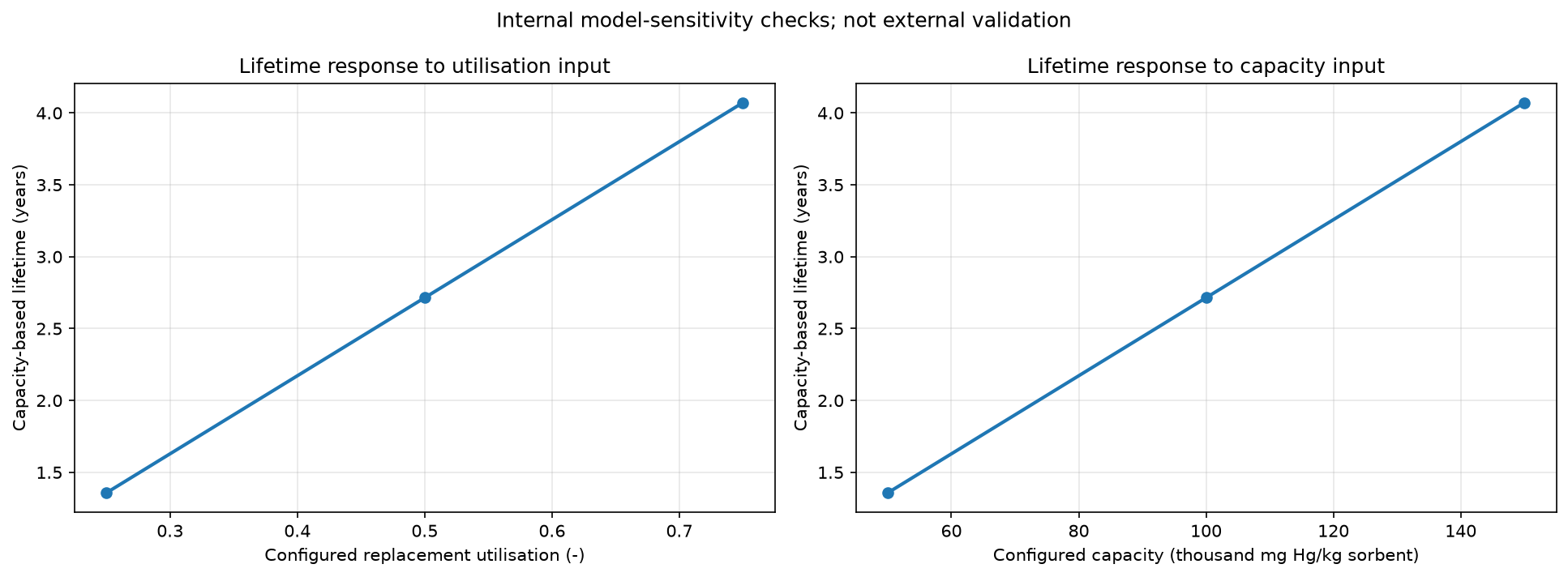
The verification below distinguishes inputs from calculations and checks internal invariants rather than counting configured values as agreement with literature.

Quantity	Evidence class
diameter, length, void fraction, particle size	configured input
bulk density, capacity, kinetic constants	configured input requiring supplier calibration
removal efficiency and pressure drop	calculated by current NeqSim implementation
sorbent mass and lifetime	algebraic consequences of geometry, capacity, flow, and utilisation
transient loading profiles	calculated response of the discretized demonstration model
wall thickness, weights, cost	preliminary screening correlations and factors

The sensitivity checks prove finite/bounded results and expected directionality for this exact case; they do not establish predictive accuracy. Public context sources are provided at the end of the notebook. No proprietary product data or uncited plant case is used as a benchmark.

def lifetime_case(name, replacement_utilisation=0.50, capacity_mg_per_kg=100000.0):
    bed = MercuryRemovalBed(name, feed)
    bed.setBedDiameter(2.0)
    bed.setBedLength(5.0)
    bed.setVoidFraction(0.40)
    bed.setParticleDiameter(0.004)
    bed.setSorbentType("PuraSpec")
    bed.setSorbentBulkDensity(1100.0)
    bed.setMaxMercuryCapacity(float(capacity_mg_per_kg))
    bed.setReactionRateConstant(0.5)
    bed.setActivationEnergy(25000.0)
    bed.setReferenceTemperature(298.15)
    bed.setReplacementUtilisation(float(replacement_utilisation))
    bed.run(UUID.randomUUID())
    return float(bed.estimateBedLifetime()) / 8760.0


utilisation_cases = np.array([0.25, 0.50, 0.75])
utilisation_lifetimes = np.array(
    [lifetime_case(f"utilisation-{value}", replacement_utilisation=value)
     for value in utilisation_cases]
)

capacity_cases = np.array([50000.0, 100000.0, 150000.0])
capacity_lifetimes = np.array(
    [lifetime_case(f"capacity-{value}", capacity_mg_per_kg=value)
     for value in capacity_cases]
)

verification_checks = {
    "steady removal is bounded": 0.0 <= removal_efficiency <= 1.0,
    "pressure drop is finite and non-negative": (
        np.isfinite(pressure_drop_bar) and pressure_drop_bar >= 0.0
    ),
    "transient time is strictly increasing": bool(np.all(np.diff(times) > 0.0)),
    "transient utilisation is non-decreasing": bool(np.all(np.diff(utilisations) >= -1.0e-12)),
    "degradation scenarios do not increase removal": bool(
        np.all(np.diff(efficiencies) <= 1.0e-10)
    ),
    "lifetime increases with replacement utilisation": bool(
        np.all(np.diff(utilisation_lifetimes) > 0.0)
    ),
    "lifetime increases with configured capacity": bool(
        np.all(np.diff(capacity_lifetimes) > 0.0)
    ),
    "normal-basis mercury conversion is reproducible": bool(
        np.isclose(
            c_hg_ntp,
            x_hg * normal_molar_density * mercury_molar_mass * 1.0e6,
            rtol=1.0e-12,
        )
    ),
}

print("=== Internal verification checks ===")
for check_name, passed in verification_checks.items():
    print(f"{'PASS' if passed else 'FAIL'}: {check_name}")

assert all(verification_checks.values())

Output

``` === Internal verification checks === PASS: steady removal is bounded PASS: pressure drop is finite and non-negative PASS: transient time is strictly increasing PASS: transient utilisation is non-decreasing PASS: degradation scenarios do not increase removal PASS: lifetime increases with replacement utilisation PASS: lifetime increases with configured capacity PASS: normal-basis mercury conversion is reproducible ```

fig, axes = plt.subplots(1, 2, figsize=(13, 4.8))

axes[0].plot(utilisation_cases, utilisation_lifetimes, "o-", linewidth=2)
axes[0].set_xlabel("Configured replacement utilisation (-)")
axes[0].set_ylabel("Capacity-based lifetime (years)")
axes[0].set_title("Lifetime response to utilisation input")
axes[0].grid(True, alpha=0.3)

axes[1].plot(capacity_cases / 1000.0, capacity_lifetimes, "o-", linewidth=2)
axes[1].set_xlabel("Configured capacity (thousand mg Hg/kg sorbent)")
axes[1].set_ylabel("Capacity-based lifetime (years)")
axes[1].set_title("Lifetime response to capacity input")
axes[1].grid(True, alpha=0.3)

fig.suptitle("Internal model-sensitivity checks; not external validation")
plt.tight_layout()
plt.savefig("mercury_internal_sensitivity.png", dpi=150, bbox_inches="tight")
plt.show()

Interpretation limits

• The feed and equipment dimensions are synthetic.
• The normal-volume conversion is explicit; process-volume density is not substituted for it.
• Capacity, kinetics, degradation, bypass, and replacement utilisation must be calibrated from appropriate supplier or test data before project use.
• The transient example uses an intentionally elevated mercury amount and coarse time steps.
• The mechanical and cost classes provide screening outputs only.
• No regulatory limit, occupational exposure limit, named-plant performance, or code-conformance claim is made.

Traceable public context

• Johnson Matthey mercury-removal absorbents describes commercial mercury-removal applications and explicitly directs users to supplier consultation for product and duty selection. It is not used here as quantitative validation.
• Granite, Pennline, and Hargis, Industrial & Engineering Chemistry Research 39 (2000), 1020–1029, doi:10.1021/ie990758v, reports laboratory packed-bed sorbent screening in carrier gases. Its flue-gas experiments are context, not an LNG natural-gas benchmark for this synthetic case.
• The exact implementation is the current MercuryRemovalBed.java, with screening design and cost logic in the adjacent mechanical-design and cost-estimation classes.

Summary

This notebook cleanly executes the complete public workflow:

Capability	API or evidence
steady calculation	MercuryRemovalBed.run()
transient loading	runTransient(dt, id) with stored tables and plots
axial state	getLoadingProfile() and getConcentrationProfile()
breakthrough diagnostics	isBreakthroughOccurred() and getBreakthroughTimeHours()
scenario controls	degradation, bypass, pre-loading, utilisation, and capacity inputs
serialization	toJson() outputs with explicit field units
mechanical screening	getMechanicalDesign().calcDesign()
cost-factor screening	getCostEstimate().calculateCostEstimate()
configuration checks	validateSetup()
verification	boundedness and monotonic sensitivity assertions

The saved values belong to one top-to-bottom execution. They show how the current NeqSim model responds to the declared synthetic inputs. They do not establish vendor performance, field life, pressure-vessel compliance, cost accuracy, or operating approval.