Note: This is an auto-generated Markdown version of the Jupyter notebook
processmodel_plant_optimization.ipynb. You can also view it on nbviewer or open in Google Colab.
This notebook demonstrates the agentic optimization workflow on a large multi-area
NeqSim ProcessModel — the same pattern used to optimize real offshore plants such as the
Oseberg Sture low-pressure operation model (a ~13-area ProcessModel with separation,
recompression, export and injection trains).
The Oseberg production model cannot be executed here because it depends on external,
site-specific data files. Instead we build a self-contained, representative two-area
ProcessModel (separation + recompression/export) that exercises the identical Java APIs,
so the workflow transfers one-to-one to the full plant.
What this notebook shows
| Step | API | Purpose |
|---|---|---|
| Build | ProcessModel.add(name, system) |
compose named process areas |
| Observe (empty) | getUtilizationSnapshotJson() |
utilization is zero until capacity limits exist |
| Size | autoSizeEquipment(safety) |
size every unit in every area in one call |
| Activate | applyMechanicalDesignCapacityConstraints() |
NEW: one call activates utilization across the whole plant |
| Observe (live) | getUtilizationSnapshotJson() |
bottleneck + per-unit utilization |
| Discover | getAdjustableParametersJson() |
bounded decision space |
| Optimize | getAutomation().evaluate(setpoints, unit, readbacks) |
convergence-gated optimizer step |
| Spec | Standard_ASTM_D6377 (RVP) |
export-oil quality constraint via penalty |
The heavy lifting (sizing, constraint construction, convergence, feasibility gating) happens inside Java NeqSim — Python only builds the plant, drives setpoints, and reads results.
Runtime: Use Git and JDK 17 or newer. The setup uses compiled repository classes when present; otherwise it fetches and builds the corrected documentation source from refs/pull/3597/head. Set NEQSIM_GIT_REF to validate another fixed revision. The public Python package alone does not contain all Java fixes exercised here. Run all cells from a fresh kernel.
import importlib.util
import os
import subprocess
import sys
import tempfile
from pathlib import Path

# Install Python packages with this notebook kernel. Java runs from the
# validated documentation source below, ahead of the package's bundled JAR.
required = {"neqsim": "neqsim>=3.20.0,<4", "numpy": "numpy",
            "scipy": "scipy>=1.14,<2", "matplotlib": "matplotlib", "pandas": "pandas"}
missing = [package for module, package in required.items()
           if importlib.util.find_spec(module) is None]
if missing:
    subprocess.check_call([sys.executable, "-m", "pip", "install", *missing])

candidate = Path(os.environ.get("NEQSIM_PROJECT_ROOT", Path.cwd())).resolve()
PROJECT_ROOT = next((p for p in [candidate, *candidate.parents]
                     if (p / "pom.xml").is_file()
                     and (p / "devtools/neqsim_dev_setup.py").is_file()), None)
if PROJECT_ROOT is None:
    # The public package alone predates fixes exercised by these examples.
    # Use the validated documentation PR's source; override with another fixed
    # commit or ref through NEQSIM_GIT_REF when validating a newer revision.
    source_ref = os.environ.get("NEQSIM_GIT_REF", "refs/pull/3597/head")
    PROJECT_ROOT = Path(tempfile.mkdtemp(prefix="neqsim-optimization-"))
    subprocess.check_call(["git", "init", "-q", str(PROJECT_ROOT)])
    subprocess.check_call(["git", "-C", str(PROJECT_ROOT), "remote", "add", "origin",
                           "https://github.com/equinor/neqsim.git"])
    subprocess.check_call(["git", "-C", str(PROJECT_ROOT), "fetch", "--depth", "1",
                           "origin", source_ref])
    subprocess.check_call(["git", "-C", str(PROJECT_ROOT), "checkout", "--quiet",
                           "--detach", "FETCH_HEAD"])
    print(f"Fetched NeqSim documentation source: {source_ref}")

if not (PROJECT_ROOT / "target/classes/neqsim/thermo/system/SystemSrkEos.class").is_file():
    # Requires Git and JDK 17+ before the first source build.
    # The Maven wrapper downloads its own Maven distribution and dependencies.
    wrapper = "mvnw.cmd" if os.name == "nt" else "mvnw"
    build = subprocess.run(
        [str(PROJECT_ROOT / wrapper), "-q", "-DskipTests", "compile",
         "dependency:build-classpath", "-DincludeScope=runtime",
         "-Dmdep.outputFile=target/neqsim-dev-classpath.txt",
         f"-Dmdep.pathSeparator={os.pathsep}"],
        cwd=PROJECT_ROOT, text=True, stdout=subprocess.PIPE, stderr=subprocess.STDOUT,
    )
    if build.returncode:
        raise RuntimeError("NeqSim source build failed:\n" + build.stdout[-12000:])

os.environ["NEQSIM_PROJECT_ROOT"] = str(PROJECT_ROOT)
sys.path.insert(0, str(PROJECT_ROOT / "devtools"))
from neqsim_dev_setup import neqsim_init, neqsim_classes
ns = neqsim_classes(neqsim_init(project_root=PROJECT_ROOT,
                              recompile=False, verbose=False))
NEQSIM_MODE = "workspace target/classes"
from neqsim import jneqsim
import numpy as np
import matplotlib.pyplot as plt

FIGURES_DIR = Path("figures")
FIGURES_DIR.mkdir(exist_ok=True)

def save_figure(filename):
    plt.savefig(FIGURES_DIR / filename, dpi=150, bbox_inches="tight")
    plt.show()

print(f"NeqSim source: {NEQSIM_MODE}")
Output
``` All NeqSim classes imported OK NeqSim source: workspace target/classes ```import json
import numpy as np
import jpype
SystemSrkEos = ns.SystemSrkEos
ProcessSystem = ns.ProcessSystem
ProcessModel = ns.ProcessModel
Stream = ns.Stream
Separator = ns.JClass("neqsim.process.equipment.separator.ThreePhaseSeparator")
Compressor = ns.Compressor
Cooler = ns.Cooler
Heater = ns.Heater
Mixer = ns.Mixer
ThrottlingValve = ns.ThrottlingValve
Standard_ASTM_D6377 = ns.JClass("neqsim.standards.oilquality.Standard_ASTM_D6377")
HashMap = ns.JClass("java.util.HashMap")
ArrayList = ns.JClass("java.util.ArrayList")
JDouble = ns.JClass("java.lang.Double")
def j(obj):
"""Parse a NeqSim JSON return value (java.lang.String) into a Python object."""
return json.loads(str(obj))
print("Classes imported")
Output
``` Classes imported ```1. Build the multi-area plant
Two process areas, composed into a single ProcessModel:
separation— well feed → 1st-stage separator (62 bara) → oil let-down valve → oil-stabilization heater → 2nd-stage separator (3 bara). Produces stabilized export oil, HP gas (gas1) and LP gas (gas2).recompression— LP gas (gas2) is cooled and recompressed to 62 bara, mixed with HP gas (gas1), cooled, and export-compressed to 150 bara.
Cross-area streams (gas1, gas2) are shared by object reference — exactly the Oseberg
pattern where each area is a ProcessSystem and ProcessModel.run() iterates to convergence.
Both oil separators distinguish hydrocarbon liquid and water. The RVPE sample is the second separator’s oil outlet. Knockout scrubbers after gas cooling prevent condensed liquid being sent into either compressor. Their liquid outlets leave the example as drain products. The LP recompressor is a lumped thermodynamic unit for this API example; detailed design requires appropriate compression stages, intercooling, discharge-temperature limits and vendor qualification.
def make_feed(rate_kghr=100000.0):
    fluid = SystemSrkEos(273.15 + 60.0, 62.0)
    for comp, x in [
        ("methane", 0.70),
        ("ethane", 0.08),
        ("propane", 0.05),
        ("n-butane", 0.04),
        ("n-pentane", 0.03),
        ("n-hexane", 0.03),
        ("n-octane", 0.04),
        ("water", 0.03),
    ]:
        fluid.addComponent(comp, x)
    fluid.setMixingRule("classic")
    fluid.setMultiPhaseCheck(True)
    feed = Stream("well feed", fluid)
    feed.setFlowRate(rate_kghr, "kg/hr")
    feed.setTemperature(60.0, "C")
    feed.setPressure(62.0, "bara")
    return feed


def build_plant(oil_heater_temp_C=65.0, export_pressure_bara=150.0):
    feed = make_feed()

    # ---- Area A: separation ----
    sep1 = Separator("first stage separator", feed)
    oil_valve = ThrottlingValve("oil let-down valve", sep1.getOilOutStream())
    oil_valve.setOutletPressure(3.0)
    oil_heater = Heater("oil stabilization heater", oil_valve.getOutletStream())
    oil_heater.setOutTemperature(oil_heater_temp_C, "C")
    sep2 = Separator("second stage separator", oil_heater.getOutletStream())

    gas1 = sep1.getGasOutStream()
    gas2 = sep2.getGasOutStream()

    separation = ProcessSystem()
    separation.setName("separation")
    for u in [feed, sep1, oil_valve, oil_heater, sep2]:
        separation.add(u)

    # ---- Area B: recompression + export ----
    recomp_cooler = Cooler("recompression cooler", gas2)
    recomp_cooler.setOutTemperature(30.0, "C")
    recomp_scrubber = Separator("recompression scrubber", recomp_cooler.getOutletStream())
    recomp = Compressor("recompression compressor", recomp_scrubber.getGasOutStream())
    recomp.setOutletPressure(62.0)
    recomp.setPolytropicEfficiency(0.78)
    recomp.setUsePolytropicCalc(True)

    mixer = Mixer("hp gas mixer")
    mixer.addStream(gas1)
    mixer.addStream(recomp.getOutletStream())

    export_cooler = Cooler("export cooler", mixer.getOutletStream())
    export_cooler.setOutTemperature(30.0, "C")
    export_scrubber = Separator("export scrubber", export_cooler.getOutletStream())
    export_comp = Compressor("export compressor", export_scrubber.getGasOutStream())
    export_comp.setOutletPressure(export_pressure_bara)
    export_comp.setPolytropicEfficiency(0.78)
    export_comp.setUsePolytropicCalc(True)

    recompression = ProcessSystem()
    recompression.setName("recompression")
    for u in [
        recomp_cooler,
        recomp_scrubber,
        recomp,
        mixer,
        export_cooler,
        export_scrubber,
        export_comp,
    ]:
        recompression.add(u)

    plant = ProcessModel()
    plant.add("separation", separation)
    plant.add("recompression", recompression)

    handles = {
        "plant": plant,
        "feed": feed,
        "sep1": sep1,
        "sep2": sep2,
        "oil_heater": oil_heater,
        "export_oil": sep2.getOilOutStream(),
        "recomp": recomp,
        "export_comp": export_comp,
    }
    return handles


P = build_plant()
plant = P["plant"]
plant.run()
print(
    "Plant converged. Areas:",
    (
        [str(a) for a in plant.getAllProcessNames()]
        if hasattr(plant, "getAllProcessNames")
        else "separation, recompression"
    ),
)
print("Export compressor power (MW):", round(float(P["export_comp"].getPower()) / 1e6, 3))
print("Recompression power (MW):    ", round(float(P["recomp"].getPower()) / 1e6, 3))
Output
``` Plant converged. Areas: separation, recompression Export compressor power (MW): 2.287 Recompression power (MW): 0.885 ```2. Utilization is empty before capacity limits exist
A freshly-built plant has no design capacity limits, so the side-effect-free
getUtilizationSnapshotJson() reports zero utilization everywhere. This is the expected
out-of-the-box state — you must give the equipment design limits before utilization means
anything.
snap_before = j(plant.getUtilizationSnapshotJson())
print("schemaVersion:", snap_before.get("schemaVersion"))
print("bottleneck:   ", snap_before.get("bottleneck"))
print("anyOverloaded:", snap_before.get("anyOverloaded"))
print("\nPer-unit maxUtilization (before sizing):")
for u in snap_before.get("units", []):
    print(
        f"  [{u.get('area','-'):>14}] {u.get('name'):<28} "
        f"{u.get('maxUtilizationPercent', 0):6.1f} %"
    )
Output
``` schemaVersion: 1.0 bottleneck: None anyOverloaded: False Per-unit maxUtilization (before sizing): [ separation] well feed 0.0 % [ separation] first stage separator 0.0 % [ separation] oil let-down valve 0.0 % [ separation] oil stabilization heater 0.0 % [ separation] second stage separator 0.0 % [ recompression] recompression cooler 0.0 % [ recompression] recompression scrubber 0.0 % [ recompression] recompression compressor 0.0 % [ recompression] hp gas mixer 0.0 % [ recompression] export cooler 0.0 % [ recompression] export scrubber 0.0 % [ recompression] export compressor 0.0 % ```3. Size the whole plant, then activate utilization in one call
autoSizeEquipment(safety)runs every area’s mechanical-design sizing tosafety× the current duty.applyMechanicalDesignCapacityConstraints()— the new bulk helper — walks every area and every unit, converts each unit’s mechanical-design limits into liveCapacityConstraints, and returns how many were registered. One call lights up utilization across the entire plant. It is idempotent (stable constraint names), so it is safe to call after every re-size.
# Size every unit for the worst-case (hottest) operating point in the sweep so the design
# ratings cover the whole optimization range, then restore the baseline setpoint.
P["oil_heater"].setOutTemperature(95.0, "C")
plant.run()
n_sized = plant.autoSizeEquipment(1.20)  # size to 120% of the worst-case duty
P["oil_heater"].setOutTemperature(65.0, "C")

# autoSizeEquipment generates a performance chart for each compressor and switches it into
# chart-based speed-solving mode (setSolveSpeed(true)). We model these machines as chartless
# (fixed outlet pressure + polytropic efficiency), so we turn the chart and speed-solving back
# off and rebuild each compressor's constraints as power-driven. We keep the mechanical-design
# power rating that autoSize assigned.
for comp in [P["recomp"], P["export_comp"]]:
    try:
        chart = comp.getCompressorChart()
        if chart is not None:
            chart.setUseCompressorChart(False)
    except Exception:
        pass
    comp.setSolveSpeed(False)
    comp.powerSet = False  # recompute duty from pressure and efficiency
    comp.setUsePolytropicCalc(True)
    comp.reinitializeCapacityConstraints()

plant.run()
n_constraints = plant.applyMechanicalDesignCapacityConstraints()
print(f"autoSizeEquipment sized {n_sized} units")
print(
    f"applyMechanicalDesignCapacityConstraints registered {n_constraints} constraints plant-wide"
)

snap = j(plant.getUtilizationSnapshotJson())
print("\nbottleneck:", snap.get("bottleneck"))
print("Per-unit maxUtilization (after sizing + activation):")
for u in snap.get("units", []):
    print(
        f"  [{u.get('area','-'):>14}] {u.get('name'):<28} "
        f"{u.get('maxUtilizationPercent', 0):6.1f} %  limit={u.get('limitingConstraint')}"
    )
Output
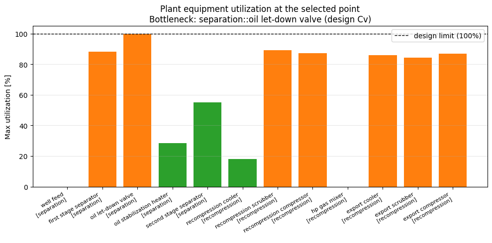
``` autoSizeEquipment sized 10 units applyMechanicalDesignCapacityConstraints registered 12 constraints plant-wide bottleneck: {'name': 'oil let-down valve', 'area': 'separation', 'qualifiedName': 'separation::oil let-down valve', 'utilization': 1.0, 'utilizationPercent': 100.0, 'limitingConstraint': 'design Cv'} Per-unit maxUtilization (after sizing + activation): [ separation] well feed 0.0 % limit=None [ separation] first stage separator 88.0 % limit=design volume flow [ separation] oil let-down valve 100.0 % limit=design Cv [ separation] oil stabilization heater 34.4 % limit=duty [ separation] second stage separator 58.4 % limit=design volume flow [ recompression] recompression cooler 24.2 % limit=duty [ recompression] recompression scrubber 89.8 % limit=gasLoadFactor [ recompression] recompression compressor 87.4 % limit=design volume flow [ recompression] hp gas mixer 0.0 % limit=None [ recompression] export cooler 86.3 % limit=duty [ recompression] export scrubber 84.4 % limit=design volume flow [ recompression] export compressor 83.2 % limit=design volume flow ```4. Tighten a real machine limit to create a clear bottleneck
Chartless compressors (defined only by an outlet pressure + efficiency) have no surge/stonewall curve, so their utilization is driven by shaft power. We give the export compressor an explicit design-power rating, then re-activate constraints. The plant now has a meaningful power-based bottleneck — exactly the situation an optimizer must respect.
# Rate the export compressor driver at a value close to its current load to expose a bottleneck.
export_power_kW = float(P["export_comp"].getPower()) / 1000.0
rated_kW = export_power_kW * 1.15
P["export_comp"].getMechanicalDesign().setMaxDesignPower(rated_kW)
P["recomp"].getMechanicalDesign().setMaxDesignPower(
    float(P["recomp"].getPower()) / 1000.0 * 1.4
)

plant.applyMechanicalDesignCapacityConstraints()  # idempotent re-activation
snap = j(plant.getUtilizationSnapshotJson())
print(f"Export compressor rated at {rated_kW:.0f} kW (current load {export_power_kW:.0f} kW)")
print("bottleneck:", snap.get("bottleneck"))
for u in snap.get("units", []):
    if u.get("maxUtilizationPercent", 0) > 1.0:
        print(
            f"  [{u.get('area','-'):>14}] {u.get('name'):<28} "
            f"{u.get('maxUtilizationPercent', 0):6.1f} %  "
            f"({u.get('limitingConstraint')})"
        )
Output
``` Export compressor rated at 2630 kW (current load 2287 kW) bottleneck: {'name': 'oil let-down valve', 'area': 'separation', 'qualifiedName': 'separation::oil let-down valve', 'utilization': 1.0, 'utilizationPercent': 100.0, 'limitingConstraint': 'design Cv'} [ separation] first stage separator 88.0 % (design volume flow) [ separation] oil let-down valve 100.0 % (design Cv) [ separation] oil stabilization heater 34.4 % (duty) [ separation] second stage separator 58.4 % (design volume flow) [ recompression] recompression cooler 24.2 % (duty) [ recompression] recompression scrubber 89.8 % (gasLoadFactor) [ recompression] recompression compressor 87.4 % (design volume flow) [ recompression] export cooler 86.3 % (duty) [ recompression] export scrubber 84.4 % (design volume flow) [ recompression] export compressor 87.0 % (power) ```6. Closed-loop optimization with evaluate()
getAutomation().evaluate(setpoints, unit, readbacks) applies the temperature
setpoint and checks model convergence. Each trial also checks the live capacity
snapshot and an export-oil quality calculation.
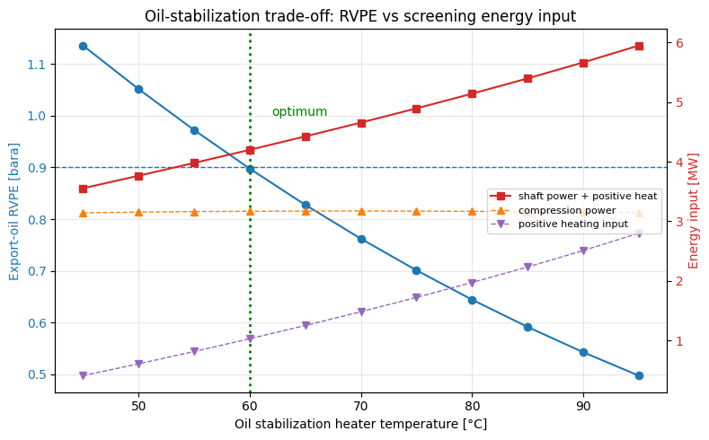
The quality metric is the ASTM D6377 RVP-equivalent estimate (RVPE) at 37.8 °C.
We explicitly select RVP_ASTM_D6377; the class default is VPCR4, a different
vapor-pressure metric. The illustrative RVPE limit is 0.90 bara.
Heating strips light ends from the oil. The optimization compares compression shaft power with positive heating input; negative heater duty is reported as cooling duty and never credited as generated power. Adding MW shaft and MW thermal is an illustrative energy-input score, not fuel consumption, exergy or electricity cost. Cooling-utility power and heater/driver efficiencies are outside this score.
We choose the best feasible sampled temperature over 45–95 °C in 5 °C steps; the result does not establish an exact continuous or global optimum.
params = j(plant.getAutomation().getAdjustableParametersJson())
print("adjustable parameter count:", params.get("count"))

# Find the heater-temperature address dynamically (robust to naming).
heater_addr = None
for p in params.get("parameters", []):
    tgt = (p.get("targetUnitName") or "").lower()
    prop = (p.get("targetProperty") or p.get("name") or "").lower()
    if "stabilization heater" in tgt and "temp" in prop:
        heater_addr = p.get("address")
        print(
            "decision variable:",
            p.get("address"),
            "| unit:",
            p.get("unit"),
            "| bounds:",
            p.get("lowerBound"),
            "->",
            p.get("upperBound"),
        )
        break

if heater_addr is None:
    # Fallback to the documented area-qualified address format.
    heater_addr = "separation::oil stabilization heater.temperature"
    print("using fallback address:", heater_addr)
Output
``` adjustable parameter count: 17 decision variable: separation::oil stabilization heater.outletTemperature | unit: C | bounds: 1.0 -> 2000.0 ```Apply the process, capacity and quality gates
A candidate must converge, accept the requested setpoint, satisfy all registered capacity limits and meet the explicitly selected RVPE specification. Failed trials are retained in the table but excluded when selecting the best operating point.
RVP_LIMIT_BARA = 0.90


def export_oil_rvp_bara():
    """ASTM D6377 RVP-equivalent estimate at 37.8 C, in bara."""
    fluid = P["export_oil"].getFluid().clone()
    std = Standard_ASTM_D6377(fluid)
    std.setReferenceTemperature(37.8, "C")
    std.setMethodRVP("RVP_ASTM_D6377")
    std.calculate()
    return float(std.getValue("RVP", "bara"))


def evaluate_trial(heater_T_C):
    """One optimizer step: set heater T, run plant, gate feasibility, read objectives."""
    sp = HashMap()
    sp.put(heater_addr, JDouble(float(heater_T_C)))
    readbacks = ArrayList()
    result = j(plant.getAutomation().evaluate(sp, "C", readbacks))

    feasible = bool(result.get("feasible"))
    rejected = result.get("setpointsRejected", {})
    # Objectives are read straight off the Java equipment after the gated run.
    p_export = float(P["export_comp"].getPower()) / 1e6
    p_recomp = float(P["recomp"].getPower()) / 1e6
    total_power = p_export + p_recomp
    heater_duty = float(P["oil_heater"].getDuty()) / 1e6  # MW (thermal)
    heating_input = max(heater_duty, 0.0)
    cooling_duty = max(-heater_duty, 0.0)
    total_energy = total_power + heating_input
    rvp = export_oil_rvp_bara()
    assert all(np.isfinite(value) for value in [total_power, heater_duty, rvp])
    snap = j(plant.getUtilizationSnapshotJson())
    overloaded = bool(snap.get("anyOverloaded"))

    return {
        "heater_T_C": heater_T_C,
        "feasible": feasible and not rejected,
        "rejected": dict(rejected) if rejected else {},
        "power_export_MW": p_export,
        "power_recomp_MW": p_recomp,
        "total_power_MW": total_power,
        "heater_duty_MW": heater_duty,
        "heating_input_MW": heating_input,
        "cooling_duty_MW": cooling_duty,
        "total_energy_MW": total_energy,
        "rvp_bara": rvp,
        "rvp_ok": rvp <= RVP_LIMIT_BARA,
        "overloaded": overloaded,
        "bottleneck": snap.get("bottleneck"),
    }


# Sweep the heater temperature across its operating band.
trials = []
for T in range(45, 96, 5):
    trials.append(evaluate_trial(float(T)))

print(
    f"{'T_C':>5} {'feas':>5} {'RVP':>6} {'ok':>4} {'P_comp':>7} {'Q_htr':>7} "
    f"{'E_tot':>7} {'overld':>7}"
)
for t in trials:
    print(
        f"{t['heater_T_C']:5.0f} {str(t['feasible']):>5} {t['rvp_bara']:6.3f} "
        f"{str(t['rvp_ok']):>4} {t['total_power_MW']:7.3f} {t['heater_duty_MW']:7.3f} "
        f"{t['total_energy_MW']:7.3f} {str(t['overloaded']):>7}"
    )
Output
``` T_C feas RVP ok P_comp Q_htr E_tot overld 45 True 1.136 False 3.143 0.411 3.554 False 50 True 1.052 False 3.154 0.610 3.764 False 55 True 0.972 False 3.163 0.816 3.979 False 60 True 0.898 True 3.169 1.030 4.199 False 65 True 0.828 True 3.172 1.253 4.425 False 70 True 0.762 True 3.172 1.484 4.656 False 75 True 0.701 True 3.171 1.724 4.895 False 80 True 0.644 True 3.167 1.974 5.141 False 85 True 0.592 True 3.162 2.235 5.397 False 90 True 0.543 True 3.156 2.510 5.665 False 95 True 0.498 True 3.148 2.801 5.949 False ```# Select only valid candidates; a penalty does not make an infeasible point feasible.
feasible_trials = [
trial
for trial in trials
if trial["feasible"] and trial["rvp_ok"] and not trial["overloaded"]
]
assert feasible_trials, "No feasible stabilization temperature in the tested range"
best = min(feasible_trials, key=lambda trial: trial["total_energy_MW"])
assert best["total_energy_MW"] >= best["total_power_MW"]
print("Best feasible sampled temperature (compression plus positive heating input):")
print(f" oil heater temperature : {best['heater_T_C']:.0f} C")
print(f" export-oil RVPE : {best['rvp_bara']:.3f} bara (limit {RVP_LIMIT_BARA} bara)")
print(f" compression power : {best['total_power_MW']:.3f} MW")
print(f" heating input : {best['heating_input_MW']:.3f} MW thermal")
print(f" cooling duty : {best['cooling_duty_MW']:.3f} MW thermal")
print(f" screening energy sum : {best['total_energy_MW']:.3f} MW")
print(f" bottleneck : {best['bottleneck']}")
Output
``` Best feasible sampled temperature (compression plus positive heating input): oil heater temperature : 60 C export-oil RVPE : 0.898 bara (limit 0.9 bara) compression power : 3.169 MW heating input : 1.030 MW thermal cooling duty : 0.000 MW thermal screening energy sum : 4.199 MW bottleneck : {'name': 'oil let-down valve', 'area': 'separation', 'qualifiedName': 'separation::oil let-down valve', 'utilization': 1.0, 'utilizationPercent': 100.0, 'limitingConstraint': 'design Cv'} ```7. Results figures
import matplotlib.pyplot as plt

Ts = [t["heater_T_C"] for t in trials]
rvps = [t["rvp_bara"] for t in trials]
energy = [t["total_energy_MW"] for t in trials]
comp_p = [t["total_power_MW"] for t in trials]
htr_q = [t["heating_input_MW"] for t in trials]

fig, ax1 = plt.subplots(figsize=(8, 5))
ax1.set_title("Oil-stabilization trade-off: RVPE vs screening energy input")
ax1.set_xlabel("Oil stabilization heater temperature [\u00b0C]")
ax1.set_ylabel("Export-oil RVPE [bara]", color="tab:blue")
ax1.plot(Ts, rvps, "o-", color="tab:blue", label="RVP")
ax1.axhline(
    RVP_LIMIT_BARA, color="tab:blue", ls="--", lw=1, label=f"RVPE limit {RVP_LIMIT_BARA} bara"
)
ax1.tick_params(axis="y", labelcolor="tab:blue")
ax1.grid(True, alpha=0.3)

ax2 = ax1.twinx()
ax2.set_ylabel("Energy input [MW]", color="tab:red")
ax2.plot(Ts, energy, "s-", color="tab:red", label="shaft power + positive heat")
ax2.plot(Ts, comp_p, "^--", color="tab:orange", lw=1, label="compression power")
ax2.plot(Ts, htr_q, "v--", color="tab:purple", lw=1, label="positive heating input")
ax2.tick_params(axis="y", labelcolor="tab:red")
ax2.legend(loc="center right", fontsize=8)

ax1.axvline(best["heater_T_C"], color="green", ls=":", lw=2)
ax1.annotate(
    "optimum",
    xy=(best["heater_T_C"], RVP_LIMIT_BARA),
    xytext=(best["heater_T_C"] + 2, RVP_LIMIT_BARA + 0.1),
    color="green",
)
fig.tight_layout()
plt.savefig("plant_optimization_tradeoff.png", dpi=120, bbox_inches="tight")
plt.show()
# Utilization bar chart at the optimum operating point.
evaluate_trial(best["heater_T_C"])  # restore the optimum state
snap = j(plant.getUtilizationSnapshotJson())
names = [f"{u.get('name')}\n[{u.get('area','-')}]" for u in snap.get("units", [])]
utils = [u.get("maxUtilizationPercent", 0) for u in snap.get("units", [])]
colors = ["tab:red" if v > 100 else ("tab:orange" if v > 80 else "tab:green") for v in utils]

fig, ax = plt.subplots(figsize=(10, 5))
ax.bar(range(len(names)), utils, color=colors)
ax.axhline(100, color="k", ls="--", lw=1, label="design limit (100%)")
ax.set_xticks(range(len(names)))
ax.set_xticklabels(names, rotation=30, ha="right", fontsize=8)
ax.set_ylabel("Max utilization [%]")
bottleneck = snap.get("bottleneck") or {}
ax.set_title(
    "Plant equipment utilization at the selected point\n"
    f"Bottleneck: {bottleneck.get('qualifiedName', 'none')} "
    f"({bottleneck.get('limitingConstraint', 'n/a')})"
)
ax.legend()
ax.grid(True, axis="y", alpha=0.3)
fig.tight_layout()
plt.savefig("plant_optimization_utilization.png", dpi=120, bbox_inches="tight")
plt.show()
# Persist a machine-readable result summary.
results = {
    "model": "self-contained 2-area ProcessModel (separation + recompression)",
    "reference_pattern": "Oseberg Sture low-pressure operation (multi-area ProcessModel)",
    "decision_variable": {"address": heater_addr, "unit": "C", "range_C": [45, 95]},
    "rvp_limit_bara": RVP_LIMIT_BARA,
    "objective": (
        "minimise shaft power plus positive heating input "
        "subject to ASTM D6377 RVPE and capacity limits"
    ),
    "optimum": {
        "oil_heater_temperature_C": best["heater_T_C"],
        "export_oil_rvp_bara": round(best["rvp_bara"], 4),
        "total_compression_power_MW": round(best["total_power_MW"], 4),
        "heater_duty_MW": round(best["heater_duty_MW"], 4),
        "total_energy_MW": round(best["total_energy_MW"], 4),
        "bottleneck": best["bottleneck"],
    },
    "trials": trials,
    "constraints_registered": int(n_constraints),
}
with open("plant_optimization_results.json", "w", encoding="utf-8") as fh:
    json.dump(results, fh, indent=2)
print("Saved plant_optimization_results.json")
print(json.dumps(results["optimum"], indent=2))
Output
``` Saved plant_optimization_results.json { "oil_heater_temperature_C": 60.0, "export_oil_rvp_bara": 0.8977, "total_compression_power_MW": 3.1688, "heater_duty_MW": 1.0305, "total_energy_MW": 4.1993, "bottleneck": { "name": "oil let-down valve", "area": "separation", "qualifiedName": "separation::oil let-down valve", "utilization": 1.0, "utilizationPercent": 100.0, "limitingConstraint": "design Cv" } } ```Summary
This notebook demonstrated the complete plant-wide optimization workflow on a multi-area
ProcessModel:
- Build named process areas and compose them with
ProcessModel.add(). - Observe that utilization is zero until design limits exist (
getUtilizationSnapshotJson()). - Size the whole plant with
autoSizeEquipment(safety). - Activate utilization across the entire plant with a single call to the new
applyMechanicalDesignCapacityConstraints()helper (idempotent, safe to re-call). - Discover the bounded decision space with
getAdjustableParametersJson(). - Optimize with the convergence-gated
evaluate()step, gating on thefeasibleflag and handling the off-model RVP spec (Standard_ASTM_D6377) as a penalty.
For the real Oseberg model the only differences are scale (≈13 areas instead of 2) and the decision vector (export/injection compressor pressures, stage pressures, heater temperatures, compressor speeds) — every API call shown here transfers unchanged.