Effective fluid properties

Similar to mineral properties, effective fluid properties are determined by the properties of each fluid phase, saturations and a mixing model. For "normal" (Newtonian) fluids, the elastic properties are bulk modulus and density from which compressional wave velocity (Vp) can be derived.

Unlike mineral properties, the elastic properties of each fluid phase are not constants. They vary with temperature and pressure, as well as other parameters, listed in Table 1 below. Pressure in terms of fluid modelling is synonymous with formation pressure.

Fluid phase	Parameters
Brine	Salinity, percentage of NaCl, KCl, CaCl₂
Gas	Gas gravity
Oil	Gas gravity, gas/oil ratio, oil density @ standard conditions
Condensate	Gas gravity, gas/oil ratio, oil density @ standard conditions
CO₂

Table 1: Required parameters for fluid modelling.

The fluid models used in this context are simplifications compared to more complex equation-of-state models, where all components must be declared with their compositional fractions. For the purpose of effective fluid properties in sedimentary rocks, the selected models suffice.

Model selection

In the open-source version of fmu-pem, most fluid models are implementations of Batzle and Wang 1992. The CO₂ model is an implementation of Span and Wagner 1996. Proprietary models may be added to the open-source ones, which is the case at Equinor. The illustrations that are included in the documentation are produced with the Equinor internal models.

Batzle, M. and Wang, Z.: Seismic properties of pore fluids. Geophysics, vol. 57, No. 11, pp. 1396–1408.

Span, R. and Wagner, W.: A New Equation of State for Carbon Dioxide Covering the Fluid Region from the Triple-Point Temperature to 1100 K at Pressures up to 800 MPa. J. Phys. Chem. Ref. Data, vol. 25, No. 6, 1996, pp. 1509–1596.

Brine model

As listed in Table 1, salinity and composition of different salts are required for modelling of brine properties, in addition to pressure and temperature. Note that the brine model assumes single-phase behaviour, i.e. it is not a model for steam, nor ice. Values for salinity and composition are taken from isotope analysis reports. An example is shown in Figure 1. The values we require here are total dissolved solids, Na⁺, Ca²⁺ and K⁺. All are given here in unit mg/L, which is equivalent to ppm, i.e., the expected unit for salinity. Calculating the percentage of Na, Ca and K should be straightforward, as they have the same unit. Variation in composition has much less influence on the elastic properties than salinity, temperature and pressure; see Figure 2.

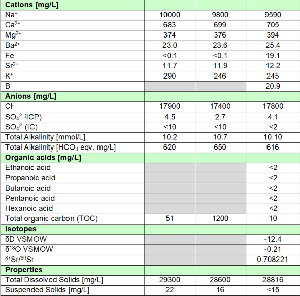Figure 1: Result of formation water isotope analysis.

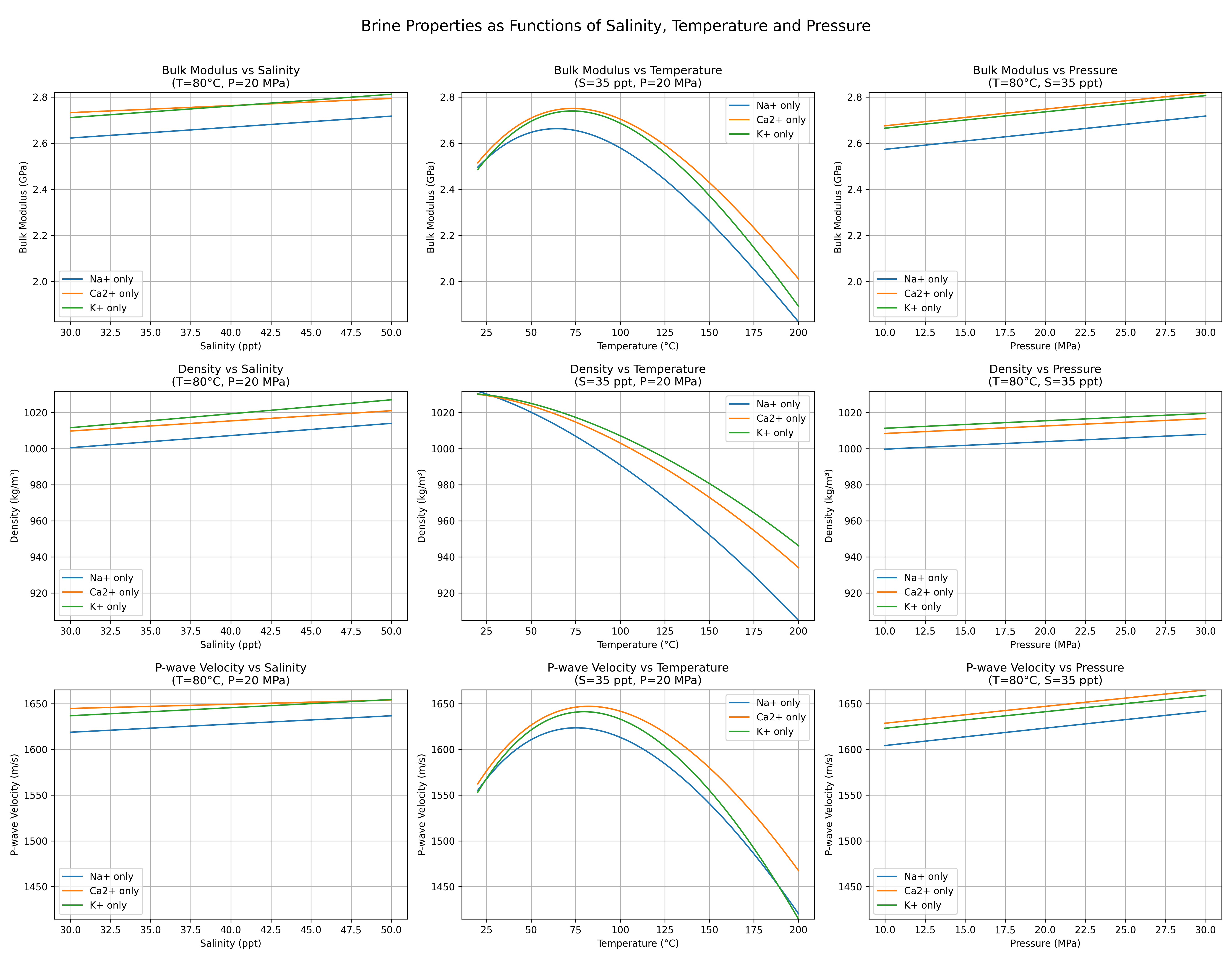Figure 2: Brine property modelling results.

Gas model

The light hydrocarbon gas model has a single parameter in addition to temperature and pressure: gas gravity. Gas gravity is defined as the molecular weight of the gas relative to the molecular weight of air. Table 2 shows the gas gravity for alkanes from methane through octane. Modelling results are shown in Figure 3.

Alkane	Chemical Formula	Molecular Weight (g/mol)	Gas Gravity (G)
Methane	CH₄	16.04	0.554
Ethane	C₂H₆	30.07	1.038
Propane	C₃H₈	44.10	1.522
Butane	C₄H₁₀	58.12	2.006
Pentane	C₅H₁₂	72.15	2.490
Hexane	C₆H₁₄	86.18	2.974
Heptane	C₇H₁₆	100.20	3.459
Octane	C₈H₁₈	114.23	3.943

Table 2: Gas gravity for different alkanes.

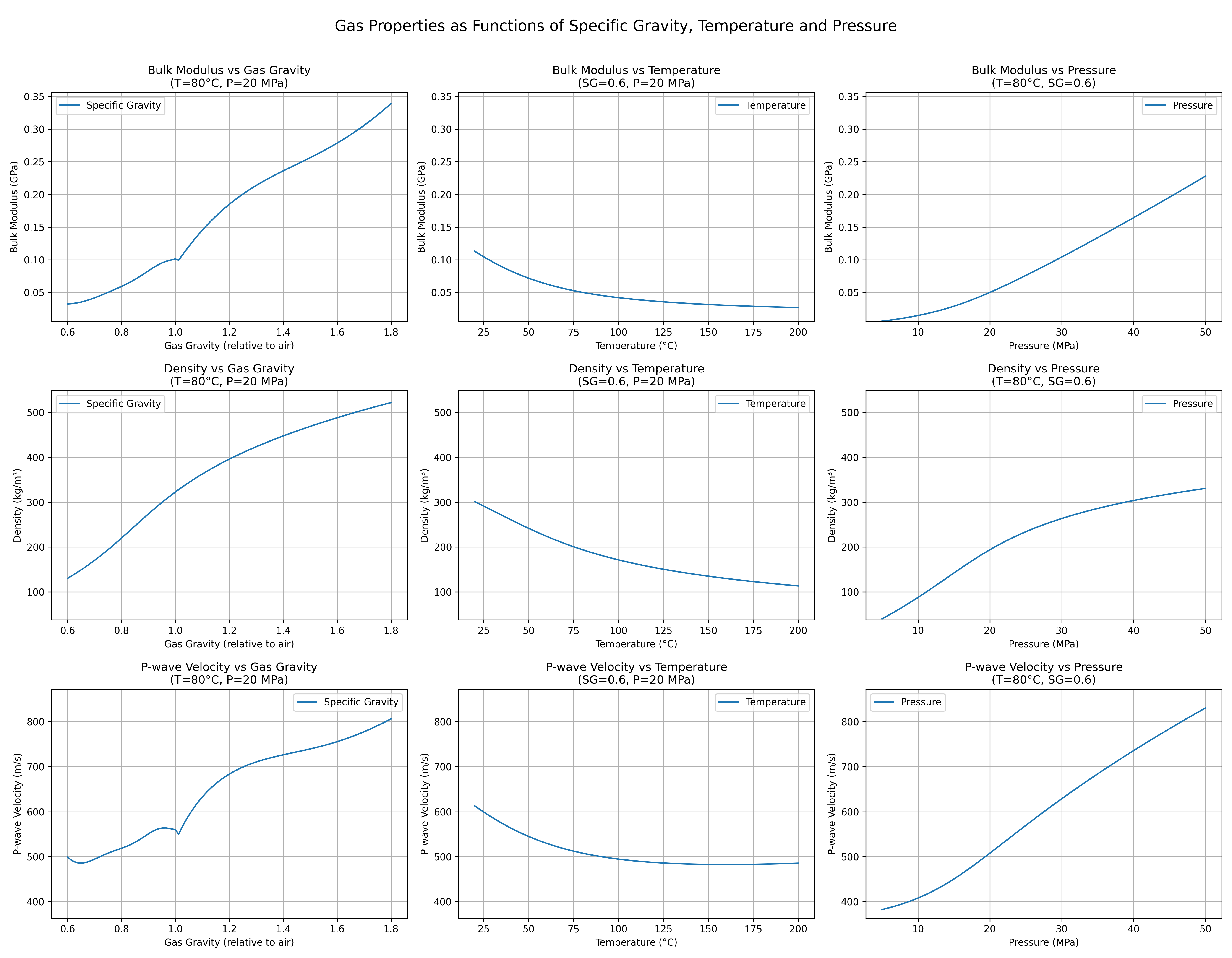Figure 3: Gas property modelling results.

Oil and condensate models

Oil and condensate models require the same set of parameters. The density of the liquid phase at standard conditions, the gravity of the gas phase and the volumetric gas/oil ratio are all required, in addition to temperature and pressure. There are limitations for most of the input parameters within a valid model range; for example, gas/oil ratio must be less than 600, otherwise the condensate model must be used.

It should also be noted that the oil model does not cover very heavy oil, such as Canadian or Venezuelan bitumen. As these varieties of hydrocarbons are not a prime target for Equinor, we have not included such models in fmu-pem. Oil with an API gravity as low as 10° can be modelled with the standard oil model, unless the temperature is very low. Oil properties as functions of temperature and pressure are shown in Figure 4. The other parameters are shown with one reference case, and comparison cases where each parameter is increased, one at a time.

In general, oil properties are reduced with increasing temperature and increased with increasing pressure. Increasing GOR reduces all oil properties, gas gravity has little influence, and increasing oil density increases all oil properties.

The oil model assumes that at reservoir conditions, all gas is dissolved in the oil. Below the bubble point, the oil model will not estimate correct results. An Equinor internal function handles cases that are below the bubble point.

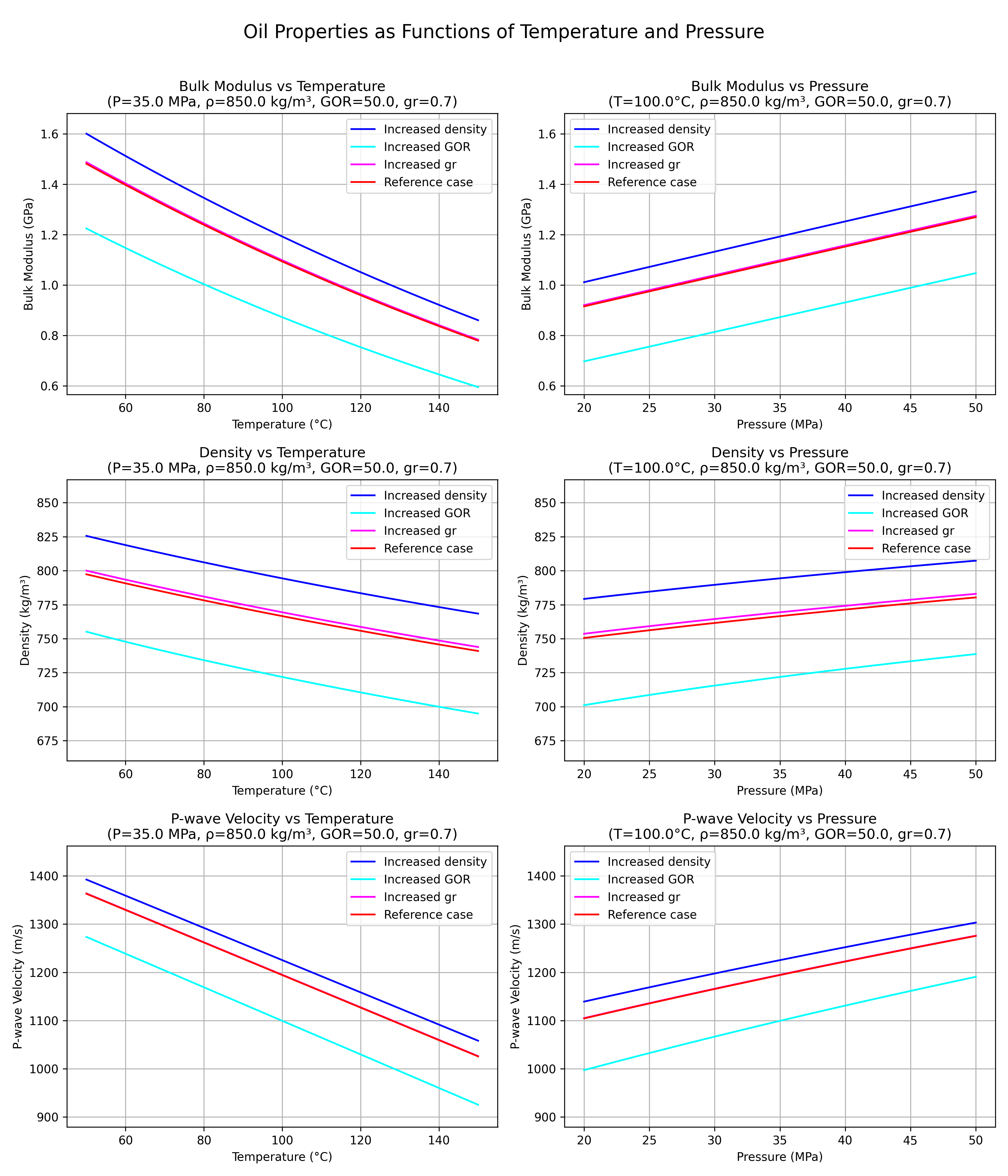Figure 4: Oil property modelling results.

CO₂ model

The CO₂ models require only temperature and pressure as parameters. The model of Span and Wagner should be the default choice, although it requires more computational time than the Equinor internal alternative. CO₂ behaviour is complex because it can exist in three different phases within normal reservoir temperature and pressure ranges: gas, liquid and supercritical phases. Figure 5 shows the CO₂ properties with one parameter varied at a time.

To get a full overview of the CO₂ properties, all combinations of reservoir temperature and pressure should be examined, as shown in Figure 6, and complemented by the phase diagram in Figure 7. Most models will not provide a complete picture of the possible combinations of hydrocarbons, brine and CO₂, as CO₂ can also react with the rock matrix and dissolve or precipitate minerals.

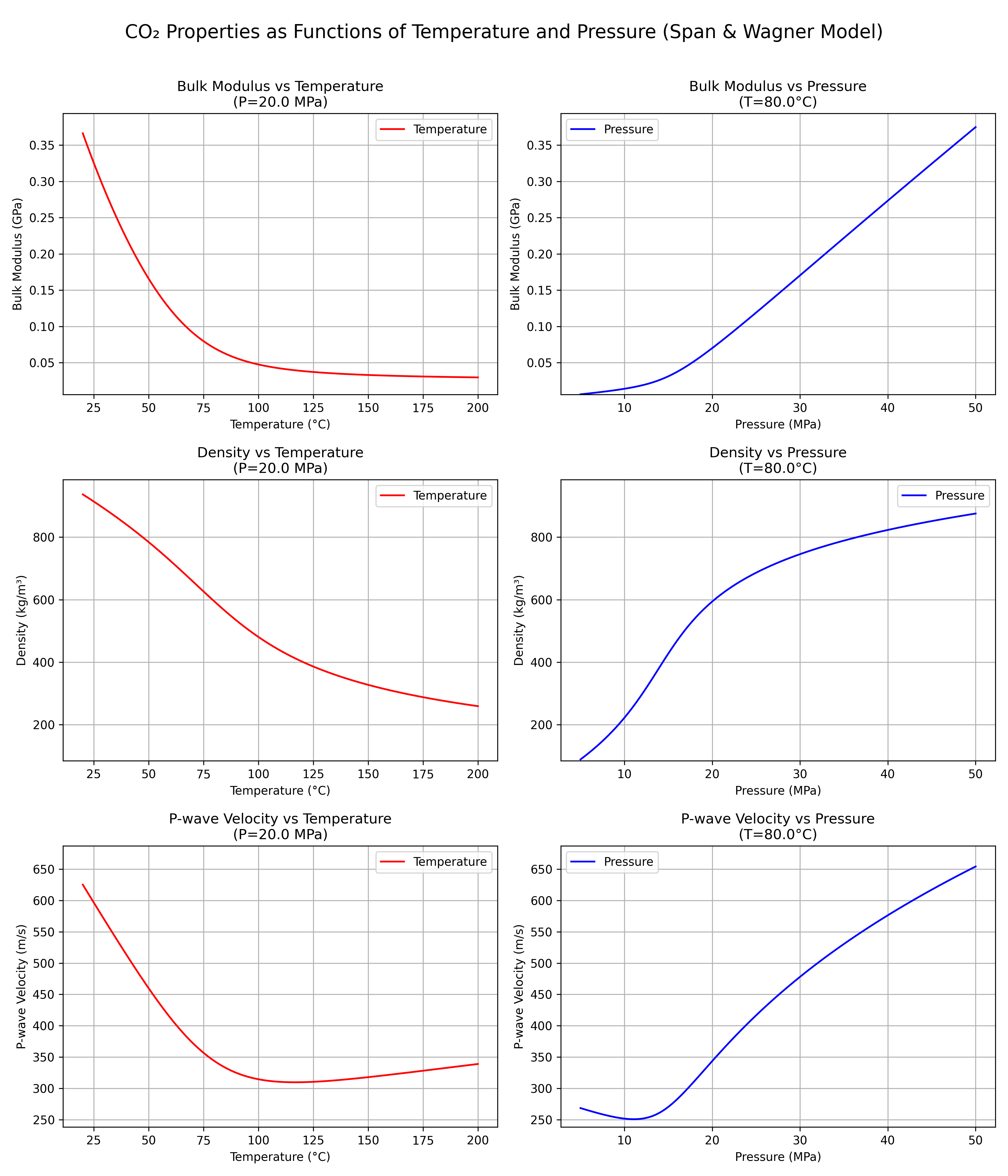Figure 5: CO₂ property modelling results.

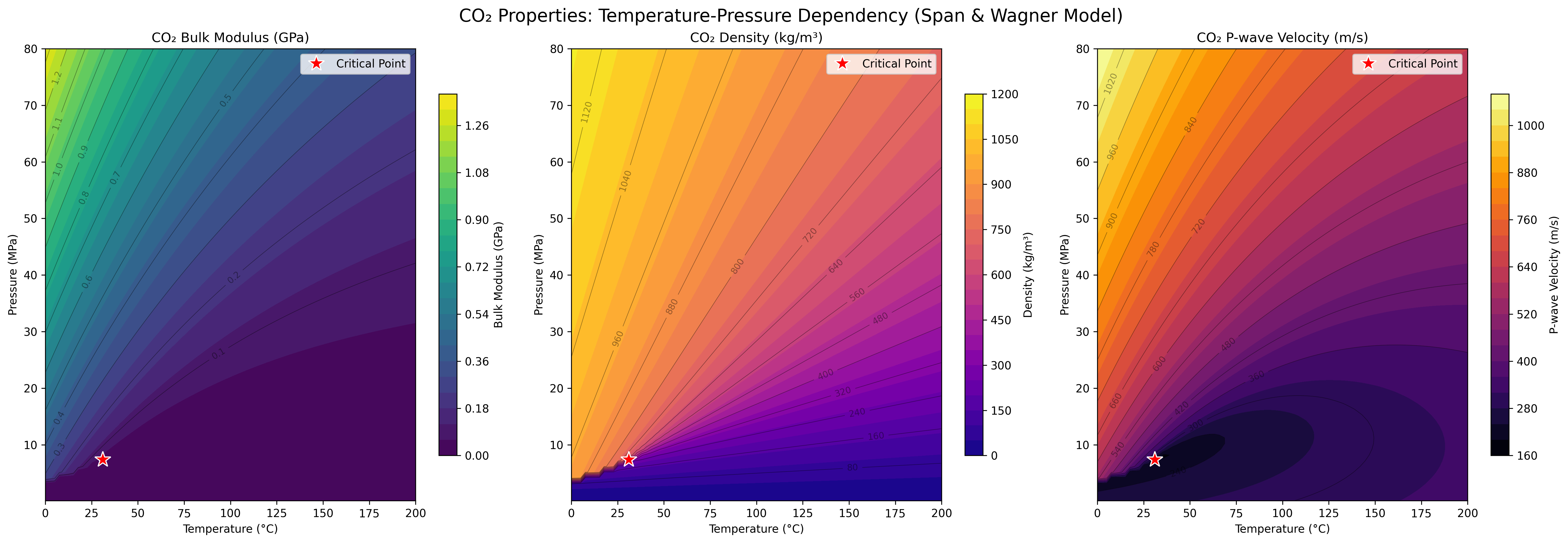Figure 6: CO₂ property modelling results.

Figure 7: CO2 phase diagram, from Yang et al. 2018.

Yang, Jianfeng & Lian, Haojie & Liang, Weiguo & Nguyen, Vinh Phu & Chen, Yuedu. (2018). Experimental investigation of the effects of supercritical carbon dioxide on fracture toughness of bituminous coals. International Journal of Rock Mechanics and Mining Sciences. 107. 10.1016/j.ijrmms.2018.04.033.

Mixing models for effective fluid properties

Two models are implemented in fmu-pem for estimating the effective fluid properties: Brie and Wood. Wood's model is similar to a Reuss lower bound, i.e. it is the softest combination of fluid phases. With Wood's model, small amounts of gas out of solution will have a strong impact on the effective fluid bulk modulus. Wood's equation assumes that fluid heterogeneities are small compared to the acoustic wavelength.

The alternative, Brie's model, is an empirical relation. It has one parameter (the Brie exponent) which determines the curve shape of the mixture. A typical value is 3.0. In a fluid mixture with more heterogeneities, Brie's model can be closer to observations than Wood's. These can be considered realistic upper and lower bounds for fluid properties , as it is unlikely that the mixture will approach the Voigt bound.

Figure 8 illustrates mixing of brine and gas. The impact of gas is most prominent in the Wood mixture. It has been noted that a small amount of gas in brine ("fizz gas") can have similar properties to oil, which has led to uncertainty in evaluation of exploration prospects.

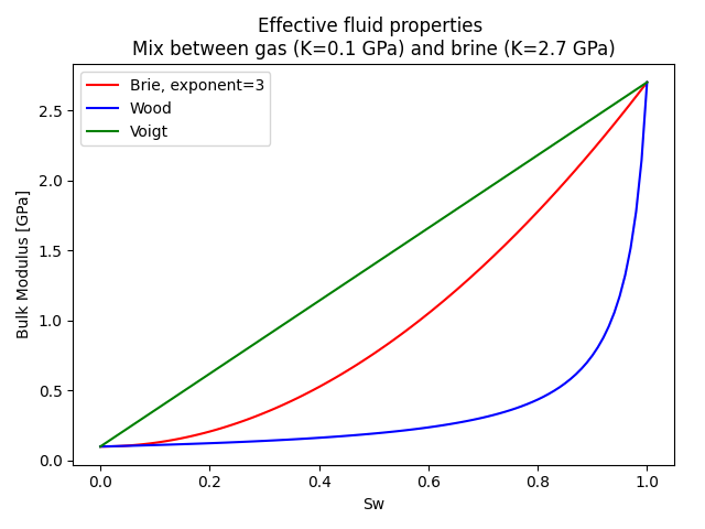Figure 8: Brine and gas mixing model comparison.

YAML file parameter settings for fluids

Most settings in the YAML config file is discussed above, expect the gas z-factor, or deviation factor for an ideal gas. This is only used in the cases where there is gas out of solution due to depletion below the bubble point of the oil. The correction for oil properties below bubble point is an Equinor internal function.

# Fluid definition: each fluid for FLAG modelling must have their parameters defined, temperature and pressure will be
# varied in the model, salinity will also be taken from model if flag is set
fluids:
  brine:
    salinity: 350000
    perc_na: 100.0
    perc_ca: 0.0
    perc_k: 0.0
  oil:
    gas_gravity: 0.763
    reference_density: 865.0
    gor: 123.0
  gas:
    type: gas
    gas_gravity: 0.763
  condensate:
    gas_gravity: 0.763
    reference_density: 865.0
    gor: 623.0

  fluid_mix_method:
    method: brie
    brie_exponent: 3.0
#    method: wood
  temperature:
    type: constant
    temperature_value: 75
#    type: from_sim
  salinity_from_sim: False
  gas_saturation_is_co2: False
  # CO2 model is either the one from FLAG or the Span-Wagner model {'flag', 'span_wagner'}
  # The FLAG model is significantly faster, but the Span-Wagner model is considered to be more accurate
  co2_model: flag
  calculate_condensate: True
  gas_z_factor: 1.0  # Factor for deviation from a ideal gas