QC using RMS
Even if sim2seis is not connected to RMS any more, the results can of course be validated within RMS if the application is available.
The results from sim2seis are attribute maps, seismic cubes and grid properties from pem. All of these data types can be imported into RMS for visual inspection and further analysis. The standard procedure is to import the data items using the RMS import menus, but an alternative is to create Python scripts that use the functionality of xtgeo.
Seismic cubes
Seismic amplitude and relative acoustic impedance cubes are saved to disk in .segy format. In the sim2seis workflow, the end results are typically difference data between two vintages of modelled seismic. The file name will contain information about which dates are the seismic base and monitor. As the seismic cubes can have time or depth as the third dimension, this information must be provided when cubes are imported into RMS.
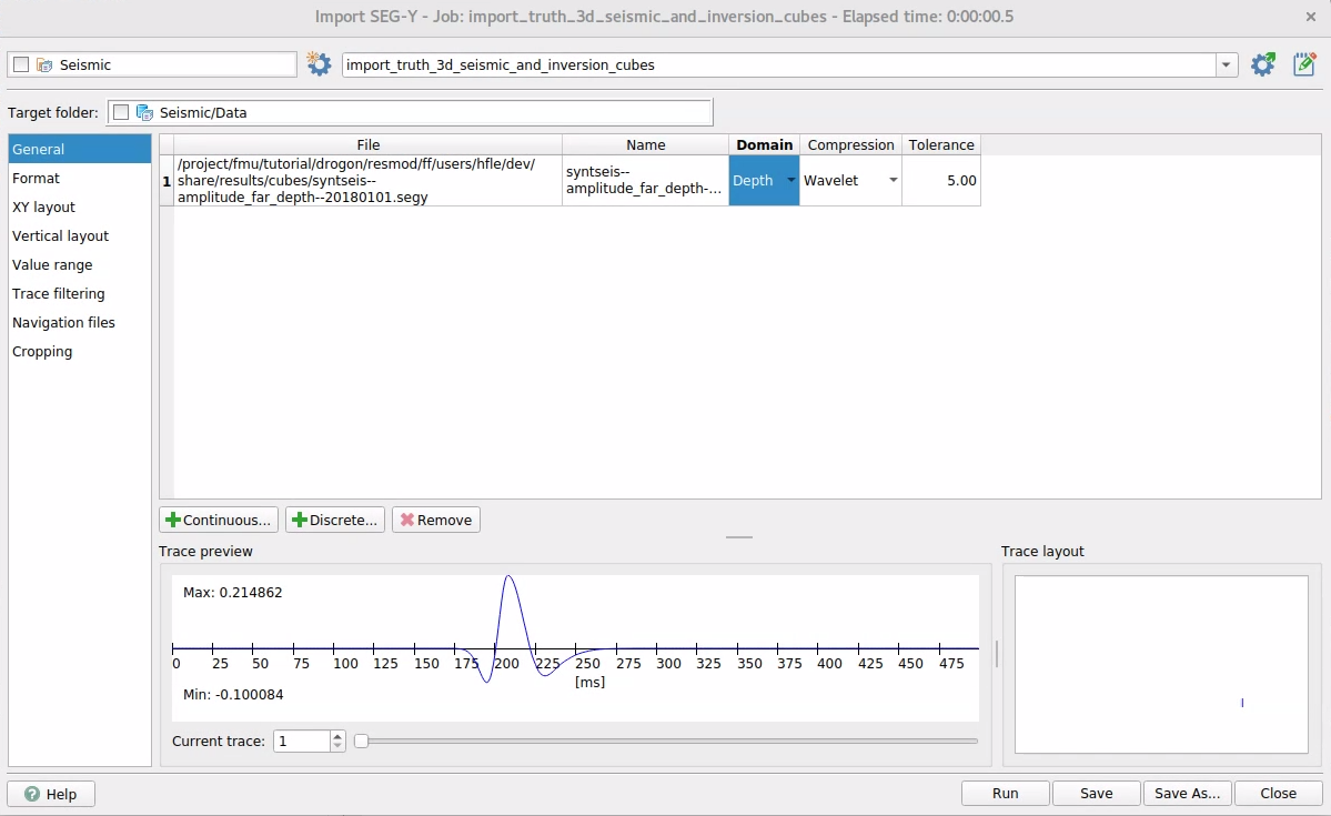 Figure 1: User dialog for cube import in RMS.
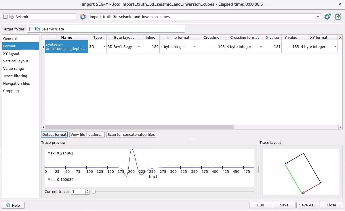 Figure 2: RMS scans for segy format and sets parameter positions.
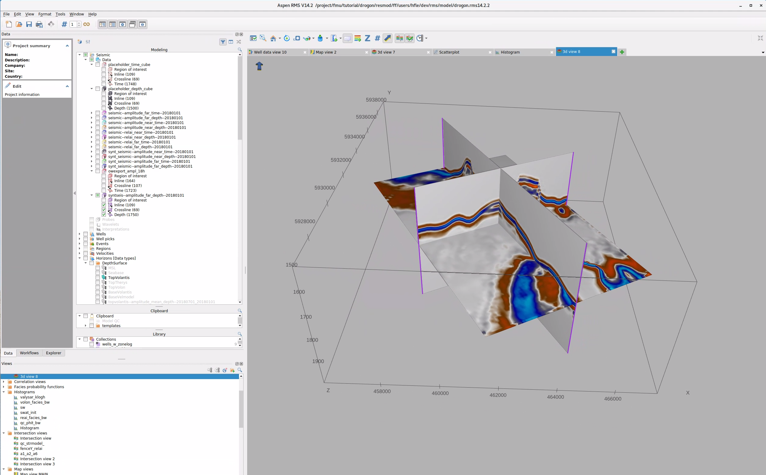 Figure 3: Visualise the cube using RMS 3D view.
All file formats saved from a sim2seis run are recognised by RMS, but instead of manual import, it might be easier to use a Python script and the xtgeo module for import. The example below is intended for running within an RMS session:
Amplitude maps
The user dialog is the same for importing to clipboard or a horizon folder in the Project data tree.
Note: attributes with low numerical values are not handled particularly well by RMS, so it may be helpful to scale values (e.g. to the thousands range).
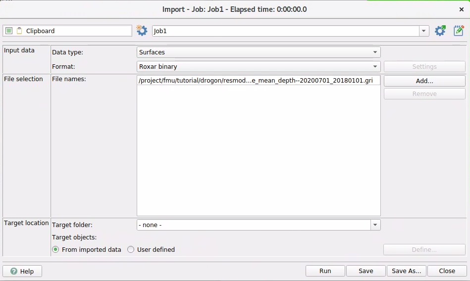 Figure 4: Attribute map import to clipboard.
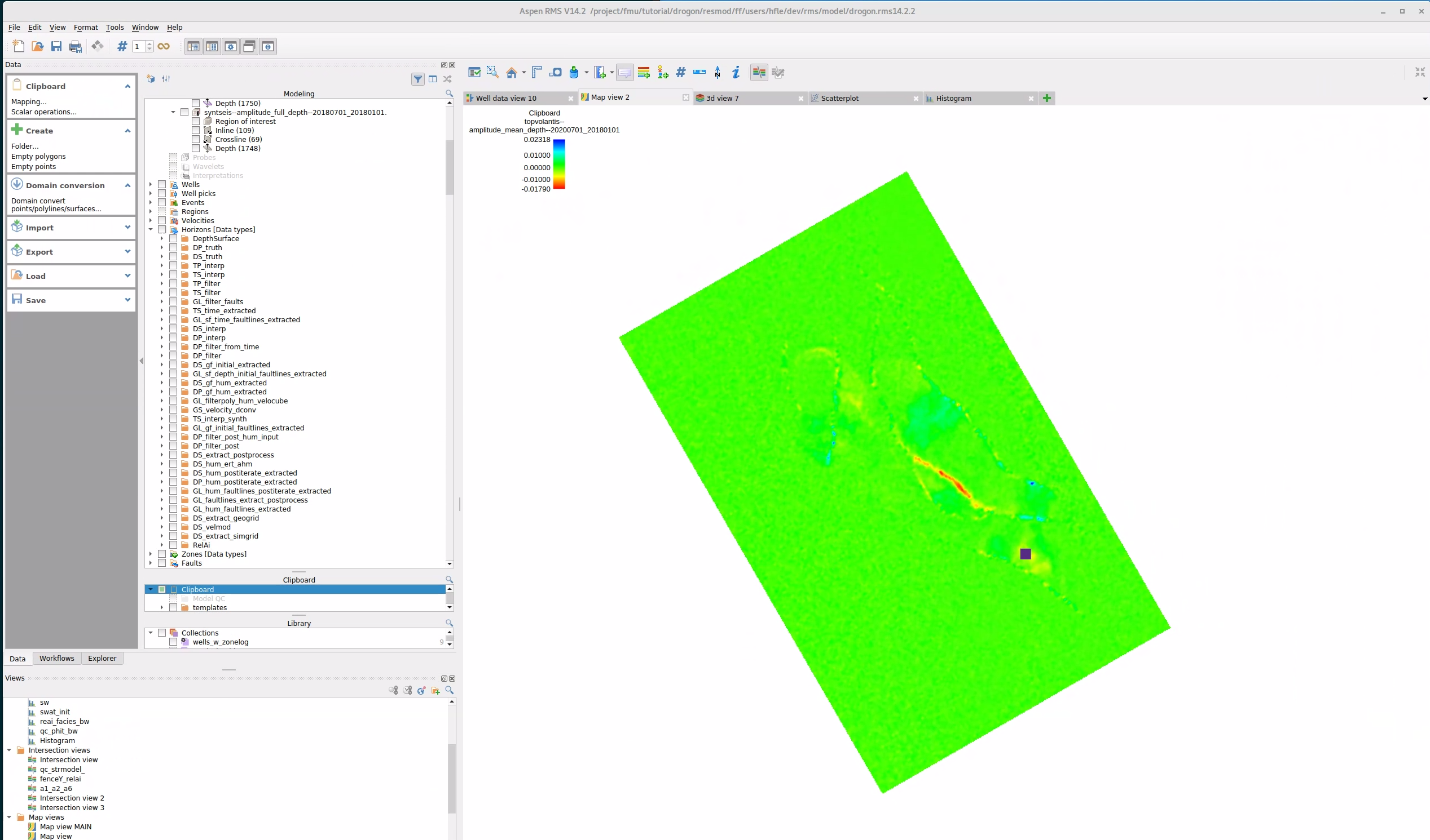 Figure 5: Visualise the attribute map. Low numerical values make the value readout insensitive.
To improve the readout of values, it is possible to scale the values in the attribute map. This can be done by multiplying the values by a factor of 1 000 000, for example. This will make the readout more accurate in the map view.
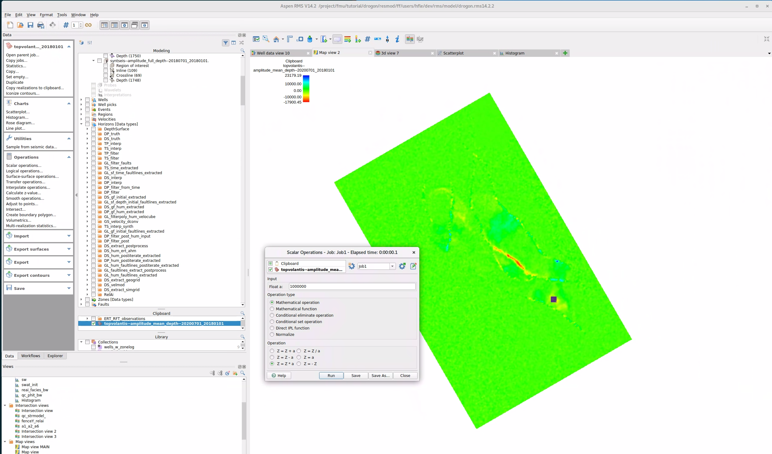 Figure 6: Boosting the values by a factor of 1 000 000 makes exact value readout more accurate.
Grid property from PEM
The grid model that the pem properties are imported to must exist before property import. Binary roff format is used for grid import. Grids are best visualised in the 3D view.
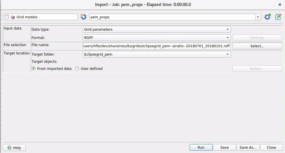 Figure 7: User dialog for grid import in RMS.
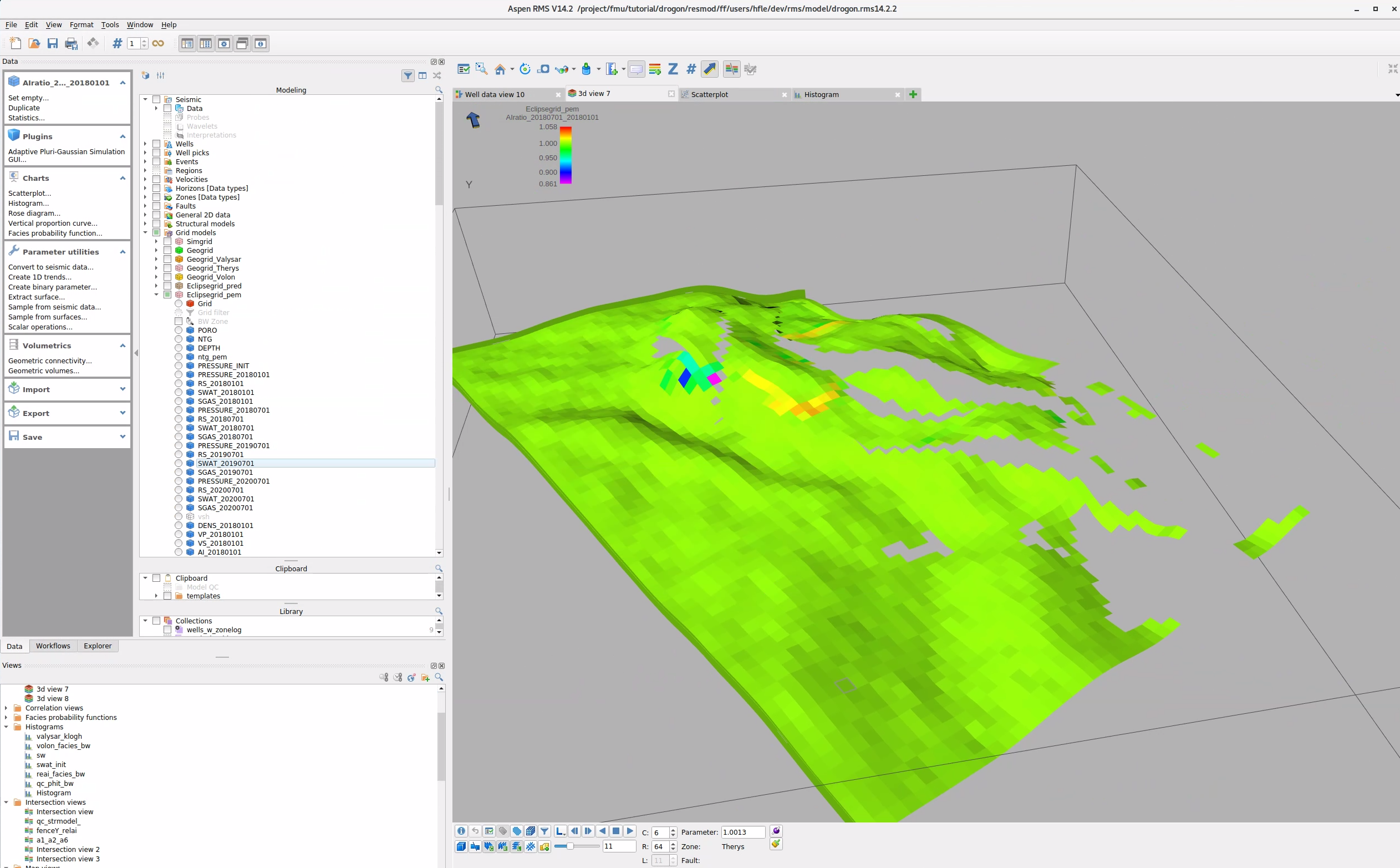 Figure 8: Grid visualisation using 3D view.
Python import script using xtgeo
Below is a Python script that illustrates how the xtgeo functionality can be used to read cube, grid and attribute map objects from file and save them to an RMS project. Note that some folders or grid models must be defined prior to running the .to_roxar(...) commands
# Import modules
import xtgeo
import os

# Reference to 'magic' project property
PRJ = project

# Directory setup
project_dir = r"/scratch/fmu/hfle/fmu_sim2seis/realization-0/iter-0"
rel_dir_obs_maps = r"share/observations/maps"
rel_dir_mod_cubes = r"share/results/cubes"
rel_dir_mod_grid = r"share/results/grids"

# Grid property import from PEM. NB! Grid model must exist before import
os.chdir(project_dir + os.path.sep + rel_dir_mod_grid)
pem_grid_name = "Eclipsegrid_pem"
pem_grid_prop_ai_name = "eclipsegrid_pem--airatio--20180701_20180101.roff"
pem_ai = xtgeo.gridproperty_from_file(pem_grid_prop_ai_name, fformat="roff")
pem_ai.to_roxar(projectname=PRJ, gridname=pem_grid_name, propertyname=pem_grid_prop_ai_name[:-4])

# Cube import
os.chdir(project_dir + os.path.sep + rel_dir_mod_cubes)
mod_amp_cube = "seismic--amplitude_full_depth--20180701_20180101.segy"
cube_amp = xtgeo.cube.cube_from_file(mod_amp_cube)
cube_amp.to_roxar(project=PRJ, name=mod_amp_cube[:-4], domain="depth")

# Map import example. NB! Note that both name and category must be defined in
# the RMS project prior to importing the map
os.chdir(project_dir + os.path.sep + rel_dir_obs_maps)
obs_relai_map = "topvolantis--relai_mean_depth--20180701_20180101.gri"
srf_ai = xtgeo.surface.surface_from_file(obs_relai_map, fformat='irap_binary')
srf_ai.to_roxar(project=PRJ, name="TopVolantis--relai--20180701-20180101", category="RelAi")