Fit an Arps curve

Here we fit a curve to data using the low-level API and plot it.

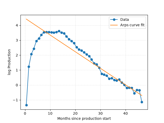
Optimal parameters are: [ 6.658  2.188 -5.326]

import matplotlib.pyplot as plt
import numpy as np
from scipy.optimize import minimize

from dca.datasets import load_monthly_sodir_production
from dca.decline_curve_analysis import Arps, CurveLoss

# Load data to fit to
df = (
    load_monthly_sodir_production()
    .loc[lambda df: df["prfInformationCarrier"] == "STATFJORD", :]
    .groupby("prfYear")["prfPrdOilNetMillSm3"]
    .sum()
)


# We fit the log-data to a log-model, and we shift the x-values
x = df.index - df.index.min() + 0.5
y = np.log(df.values)


def log_arps(t, theta1, theta2, theta3):
    """Curve function to fit to."""
    return Arps(theta1, theta2, theta3).eval_log(t)


def log_arps_grad(t, theta1, theta2, theta3):
    """Evaluate the gradient of the log of the Arps model."""
    return Arps(theta1, theta2, theta3).eval_grad_log(t)


# Prior mean and optimization first guess for parameters
mu = np.array([10, 2, 0])
# Controls prior strength
alpha = 1e-2
precision_matrix = np.eye(3) * alpha
loss_function = CurveLoss(
    mu=mu,
    precision_matrix=precision_matrix,
    curve_func=log_arps,
    curve_func_grad=log_arps_grad,
    half_life=24,
    p=1.5,
)

# Optimize the function
optimization_result = minimize(
    loss_function,
    x0=mu,
    method="BFGS",
    jac=loss_function.grad,  # Use gradient information
    args=(
        x,
        y,
    ),
)
assert optimization_result.success
optimal_parameters = optimization_result.x
print(f"Optimal parameters are: {optimal_parameters.round(3)}")


# Plot the results
plt.plot(x, y, "-o", label="Data")
curve = Arps(*optimal_parameters)
plt.plot(x, curve.eval_log(x), label="Arps curve fit")
plt.xlabel("Months since production start")
plt.ylabel("log Production")
plt.grid(True, ls="--", alpha=0.33)
plt.legend()
plt.show()