Loss function parameters

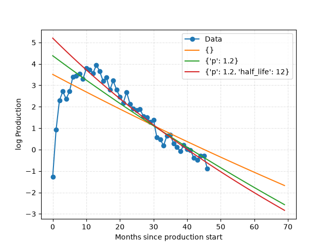
Tweaking loss function parameters.

import matplotlib.pyplot as plt
import numpy as np
from scipy.optimize import minimize

from dca.datasets import load_monthly_sodir_production
from dca.decline_curve_analysis import Arps, CurveLoss

# Load data to fit to
df = (
    load_monthly_sodir_production()
    .loc[lambda df: df["prfInformationCarrier"] == "STATFJORD", :]
    .groupby("prfYear")["prfPrdOilNetMillSm3"]
    .sum()
)

# We fit the log-data to a log-model, and we shift the x-values
rng = np.random.default_rng(42)
x = df.index - df.index.min()
x_eval = np.linspace(0, np.max(x) * 1.5)
y = np.log(df.values) + rng.normal(loc=0, scale=0.3, size=len(x))
plt.plot(x, y, "-o", label="Data")


def log_arps(t, theta1, theta2, theta3):
    """Curve function to fit to."""
    return Arps(theta1, theta2, theta3).eval_log(t)


def log_arps_grad(t, theta1, theta2, theta3):
    """Evaluate the gradient of the log of the Arps model."""
    return Arps(theta1, theta2, theta3).eval_grad_log(t)


# Default parameters
parameters = {"p": 2, "half_life": np.inf}

parameter_diffs = [
    {},  # ALl default
    {"p": 1.2},  # Median regression
    {"p": 1.2, "half_life": 12},
]

for parameter_diff in parameter_diffs:
    loss_params = {**parameters, **parameter_diff}
    mu = np.array([6, 2, 0])
    loss_function = CurveLoss(
        curve_func=log_arps,
        curve_func_grad=log_arps_grad,
        mu=mu,
        precision_matrix=np.eye(3) * 2e-1,
        **loss_params,
    )

    # Optimize the function
    optimization_result = minimize(
        loss_function,
        x0=mu,
        method="BFGS",
        jac=loss_function.grad,  # Use gradient information
        args=(
            x,
            y,
        ),
    )
    assert optimization_result.success
    optimal_parameters = optimization_result.x

    # Plot
    curve = Arps(*optimal_parameters)
    plt.plot(x_eval, curve.eval_log(x_eval), label=f"{parameter_diff}")


# Plot the results
plt.xlabel("Months since production start")
plt.ylabel("log Production")
plt.grid(True, ls="--", alpha=0.33)
plt.legend()
plt.show()