Effect of prior

We show how the prior works. As more and more data is seen, the effect of the prior lessens.

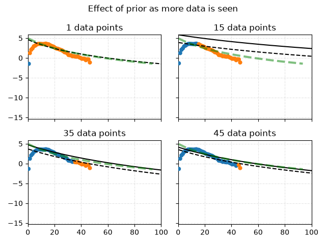
/home/runner/work/decline-curve-analysis/decline-curve-analysis/examples/plot_prior_effect.py:31: Pandas4Warning: Passing integer data to PeriodArray/PeriodIndex is deprecated and will change behavior in a future version, when integers will be treated as period ordinals instead of calendar years. To get the future behavior now, use PeriodIndex.from_ordinals(data, freq=...). To retain the current behavior, pass strings, e.g. data.astype(str).
  time = pd.PeriodIndex(series.index, freq="Y")

import itertools

import matplotlib.pyplot as plt
import numpy as np
import pandas as pd
import scipy as sp

from dca.adca.well import Well
from dca.datasets import load_monthly_sodir_production
from dca.decline_curve_analysis import Arps
from dca.models import beta_logpdf_grad, gamma_logpdf_grad

# Load data to fit to
series = (
    load_monthly_sodir_production()
    .loc[lambda df: df["prfInformationCarrier"] == "STATFJORD", :]
    .groupby("prfYear")["prfPrdOilNetMillSm3"]
    .sum()
).iloc[:]

time = pd.PeriodIndex(series.index, freq="Y")
well = Well(time=time, production=series.to_numpy())

PRIOR_MEAN = np.array([7, 2, -1])


class Prior:
    def __init__(self, prior_mean):
        self.prior_mean = np.array(prior_mean)

    def __call__(self, theta, sigma, phi, p, prior_strength):
        theta_prior = sp.stats.multivariate_normal(mean=self.prior_mean)
        sigma_prior = sp.stats.gamma(a=1.5, scale=10)
        phi_prior = sp.stats.beta(2, 2)
        p_prior = sp.stats.beta(2, 2)

        neg_log_pdf = -prior_strength * (
            theta_prior.logpdf(theta)
            + sigma_prior.logpdf(sigma)
            + phi_prior.logpdf(phi)
            + p_prior.logpdf(p - 1)
        )
        return neg_log_pdf

    def gradient(self, theta, sigma, phi, p, prior_strength):
        # Gradient
        grad_theta = self.prior_mean - theta
        grad_sigma = gamma_logpdf_grad(sigma, scale=10, a=1.5)
        grad_phi = beta_logpdf_grad(phi, a=2, b=2)
        grad_p = beta_logpdf_grad(p - 1, a=2, b=2)

        gradients = [grad_theta, grad_sigma, grad_phi, grad_p]
        # Flatten: [2, [3, 4]] => [2, 3, 4]
        chained = list(itertools.chain(*(np.atleast_1d(g) for g in gradients)))
        return -prior_strength * np.array(chained)


neg_logpdf_prior = Prior(prior_mean=PRIOR_MEAN)


fig, axes = plt.subplots(2, 2, sharex=True, sharey=True)
fig.suptitle("Effect of prior as more data is seen")
axes = iter(axes.ravel())
time = np.arange(2 * len(series)) + 0.5  # For plotting prior

# Loop over number of data points
for split in [1, 15, 35, 45]:
    ax = next(axes)

    # Plot the prior
    prior_curve = Arps(*PRIOR_MEAN)
    ax.plot(
        time,
        prior_curve.eval_log(time),
        color="green",
        zorder=99,
        alpha=0.5,
        ls="--",
        lw=3,
    )

    # Fit a Well using the desired number of data points in `split`
    well = well.fit(
        half_life=12,
        prior_strength=1,
        split=split,
        neg_logpdf_prior=neg_logpdf_prior,
    )

    # Plot the well, clean up the axis
    well.plot(split=split, logscale=True, ax=ax, q=[0.5])
    ax.set_title(f"{split} data points")
    ax.get_legend().remove()
    ax.set_xlabel("")
    ax.set_ylabel("")
    ax.set_xlim([0, 100])

fig.tight_layout()
plt.show()