Well plotting methods

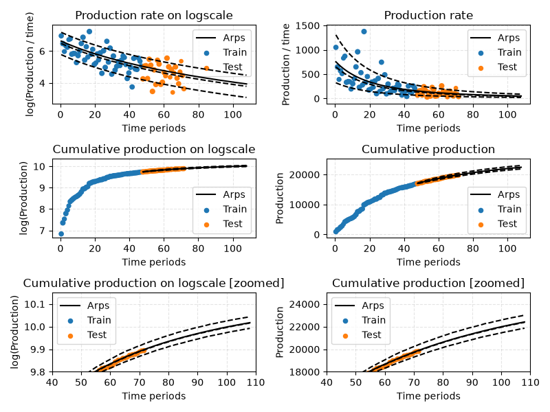
Showcases plotting capabilities.

import matplotlib.pyplot as plt

from dca.adca.well import Well

# Parameters to change
SPLIT = 0.66
curve_parameters = (10, 3.5, -1)
q = [0.1, 0.5, 0.9]
STD = 0.66

# Generate a random well and fit it
well = Well.generate_random(
    n=100,
    curve_model="arps",
    seed=2,
    preprocessing="producing_time",
    curve_parameters=curve_parameters,
    std=STD,
)
well.fit(half_life=None, prior_strength=1e-4, split=SPLIT)


# Set up plot
fig, axes = plt.subplots(3, 2, figsize=(8, 6), sharex=False)
ax1, ax2, ax3, ax4, ax5, ax6 = axes.ravel()

# Rates
well.plot(split=SPLIT, ax=ax1, logscale=True, q=q)
ax1.set_title("Production rate on logscale")

well.plot(split=SPLIT, ax=ax2, logscale=False, q=q)
ax2.set_title("Production rate")

# Cumulative production
well.plot_cumulative(split=SPLIT, ax=ax3, logscale=True, q=q)
ax3.set_title("Cumulative production on logscale")

well.plot_cumulative(split=SPLIT, ax=ax4, logscale=False, q=q)
ax4.set_title("Cumulative production")

# Zoomed in
well.plot_cumulative(split=SPLIT, ax=ax5, logscale=True, q=q)
ax5.set_title("Cumulative production on logscale [zoomed]")
ax5.set_ylim([9.8, 10.15])
ax5.set_xlim([40, 110])

well.plot_cumulative(split=SPLIT, ax=ax6, logscale=False, q=q)
ax6.set_title("Cumulative production [zoomed]")
ax6.set_ylim([1.8e4, 2.5e4])
ax6.set_xlim([40, 110])

# Relabel x-axes
for ax in axes.ravel():
    ax.set_xlabel("Time periods")

fig.tight_layout()
plt.show()