Future simulations

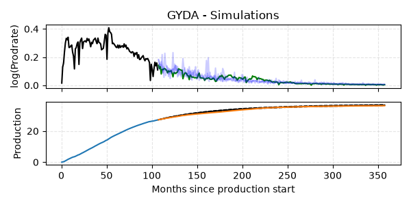
Shows how to Monte Carlo simulate the future.

{'p': np.float64(1.1750182019164204), 'sigma': np.float64(0.2658888425595641), 'phi': np.float64(0.019681858945647165), 'theta': array([ 4.02310131,  3.95211774, -1.69933228])}

import matplotlib.pyplot as plt
import numpy as np
import pandas as pd

from dca.adca.well import Well
from dca.datasets import load_monthly_sodir_production

FIELD = "GYDA"

# Read data from a public source (SODIR - sokkeldirektoratet)
df = (
    load_monthly_sodir_production()
    .loc[lambda df: df.prfInformationCarrier == FIELD, :]
    .rename(
        columns={
            "prfInformationCarrier": "field",
            "prfYear": "year",
            "prfMonth": "month",
            "prfPrdOilNetMillSm3": "production",
        }
    )
    .assign(day=1)
    .assign(
        time=lambda df: pd.to_datetime(df[["year", "month", "day"]]).dt.to_period(
            freq="M"
        )
    )
    .loc[lambda df: df.production > 0]
)


well = Well(
    production=df.production.to_numpy(),
    time=df.time,
    id=FIELD,
    preprocessing="producing_time",
    curve_model="arps",
)


# Fit the well
SPLIT = 0.3
HALF_LIFE = 12  # The uncertainty is also very dependent on half-life
well = well.fit(half_life=HALF_LIFE, prior_strength=1, split=SPLIT)
print(well.parameters_)


# Compute pre_eta, needed to initialize the simulations
(x_train, y_train, w_train), (x_test, y_test, w_test) = well.get_train_test(split=SPLIT)
preds_train = well.predict(x_train, time_on=w_train, q=0.5)
prev_eta = (np.log(y_train) - np.log(preds_train))[-1]

# Simulate a few production rates
simulations = well.simulate(
    x_test,
    time_on=w_test,
    prev_eta=prev_eta,
    seed=abs(hash(well.id)) % 2**8,
    simulations=9,
)


fig, (ax1, ax2) = plt.subplots(figsize=(6, 3), nrows=2, ncols=1, sharex=True)

# ===================== SIMULATE FUTURE PRODUCTION RATES =====================
ax1.set_title(f"{FIELD} - Simulations")
ax1.plot(x_train, y_train, color="black")
ax1.plot(x_test, y_test, color="green")


# Plot a single simulation (change to plot several)
for j in range(3):
    ax1.plot(x_test, simulations[j, :], zorder=5, color="blue", alpha=0.2)

ax1.set_ylabel("log(Prodrate)")
ax1.grid(True, ls="--", alpha=0.33)

# ===================== SIMULATE FUTURE PRODUCTION =====================

# Simuate future cumulative production
simulations = well.simulate_cumprod(
    x=x_test,
    prev_eta=prev_eta,
    seed=42,
    simulations=999,
) + np.sum(y_train * w_train)
q10, q50, q90 = np.percentile(simulations, q=[10, 50, 90], axis=0)


# Simulation results
ax2.plot(x_test, q10, lw=1, ls="--", color="black")
ax2.plot(x_test, q50, ls="-", color="black")
ax2.plot(x_test, q90, lw=1, ls="--", color="black")

# Train and test cumulatives
ax2.plot(x_train, np.cumsum(y_train * w_train))
ax2.plot(x_test, np.sum(y_train * w_train) + np.cumsum(y_test * w_test))


ax2.set_ylabel("Production")
ax2.set_xlabel("Months since production start")
ax2.grid(True, ls="--", alpha=0.33)
fig.tight_layout()
plt.show()